 |
|
|
| |
|
|
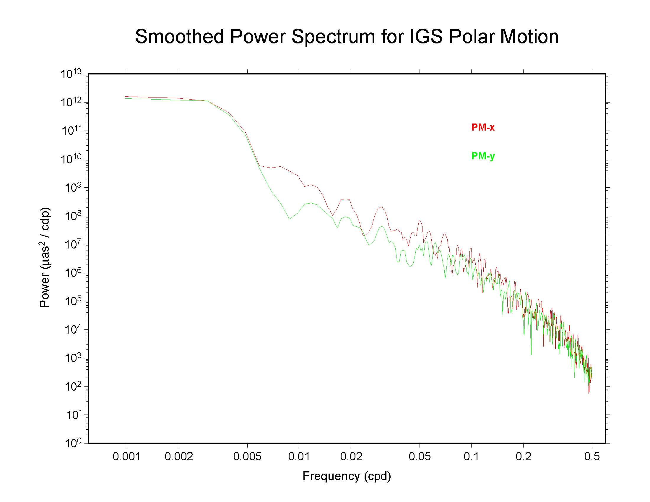
Power spectra have been generated and are plotted below for the IGS Final polar motion time series. The 1024 days from MJD 53412.5 (week 1309-5 or 11 Feb 2005) to 54435.5 (week 1455-6 or 01 Dec 2007) have been examined and a smoothing across each three adjacent frequencies applied with a sliding boxcar filter (merely to make the appearance less noisy; this is not necessary).
The spectrum for the IGS combined series (igs00p03.erp), from Remi
Ferland's SINEX combination process, is below. The smoothed spectrum
for the X component of polar motion is shown as the red curve whereas
the Y component is shown in green.
 http://www.ngs.noaa.gov/igsacc/erp/igs00p03-sm3.ps
Most continuous geophysical processes and most physical noise processes
possess power spectra that decrease as the frequency raised to some
characteristic negative power ("spectral index"). The spectra are usually
"reddish" in the sense of having more power at the lower frequencies
(i.e., longer periods).
The gradual steepening of the IGS power spectra at the highest
frequencies (approaching the Nyquist cutoff of 0.5 cpd) could indicate
some high-frequency smoothing or filtering process that dampens the
amount of energy at the shortest periods. However, one cannot reach
this inference uniquely based only on these spectra.
Power Spectra of AC Finals Polar Motion Series
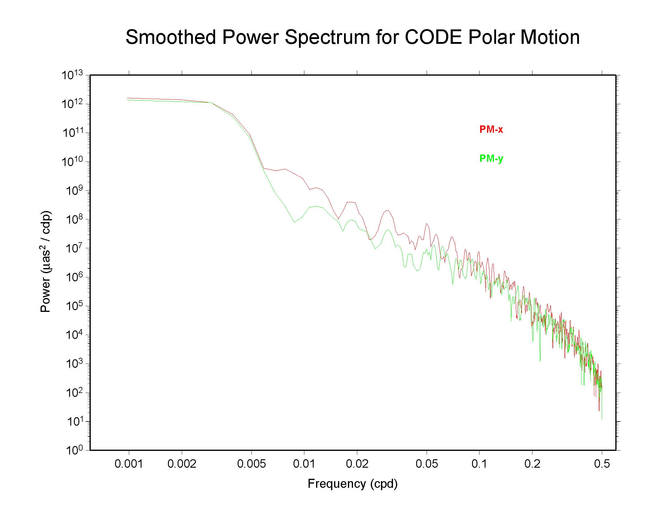
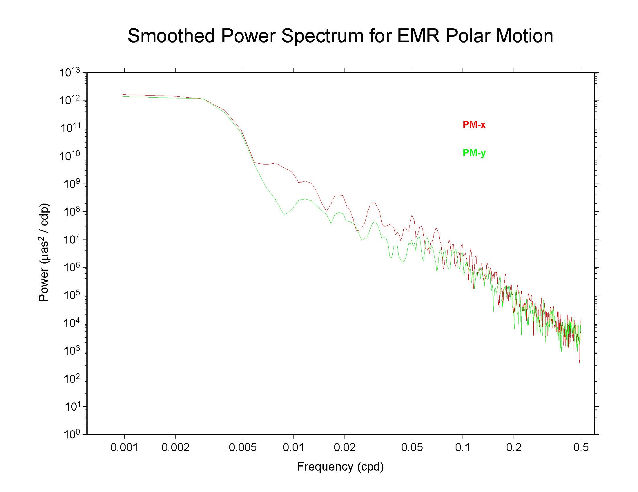
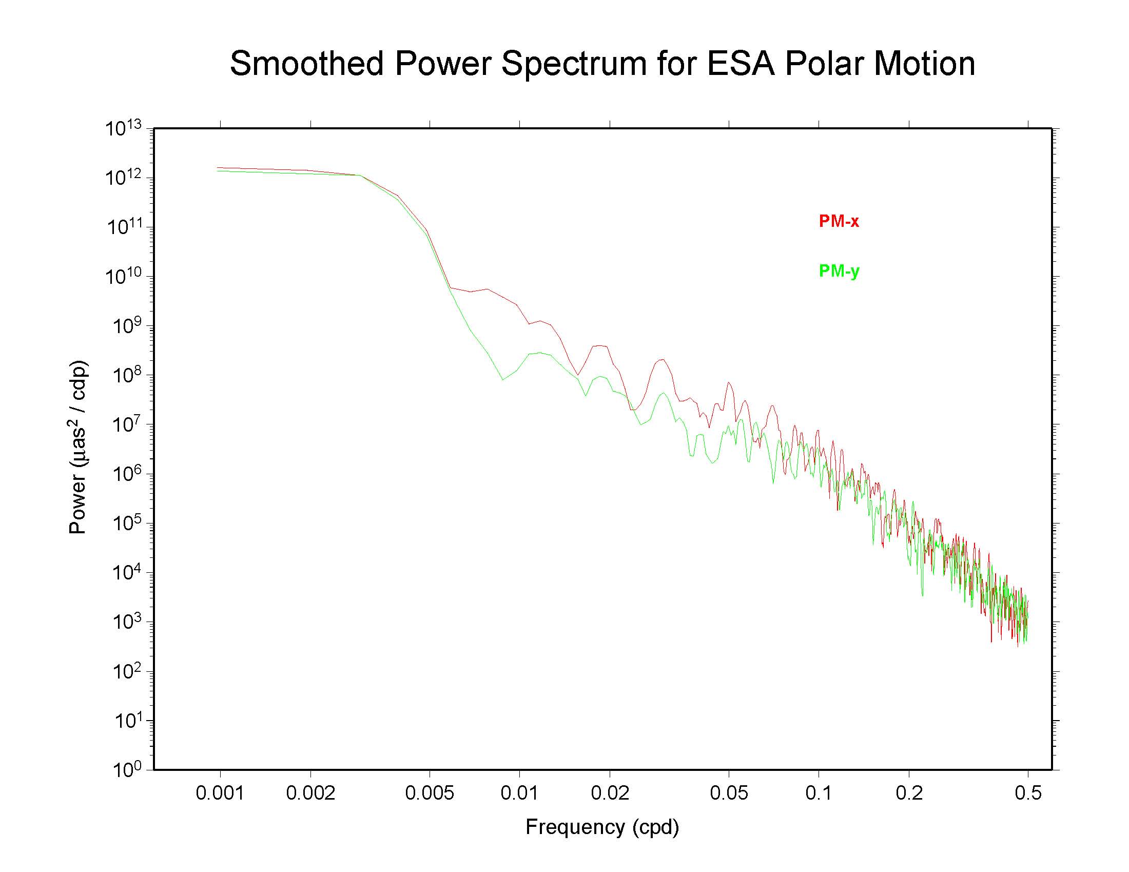
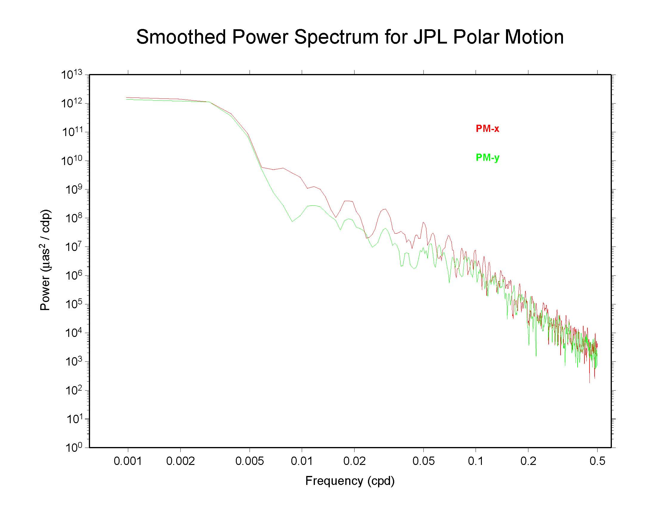
To check whether the apparent smoothing comes from any/all of the Analysis Center submissions, similar polar motion spectra have been generated for each:
Of these AC polar motion spectra, only EMR, ESA, and GFZ show completely
nominal characteristics; that is, their spectra follow a single
power-law for periods shorter than about 10 days (with spectral
index around -4) and no smoothing or excess noise is evident.
JPL and SIO show nearly power-law behavior, but both probably also display
the effects of a modest white noise floor as frequencies approach 0.5 cpd.
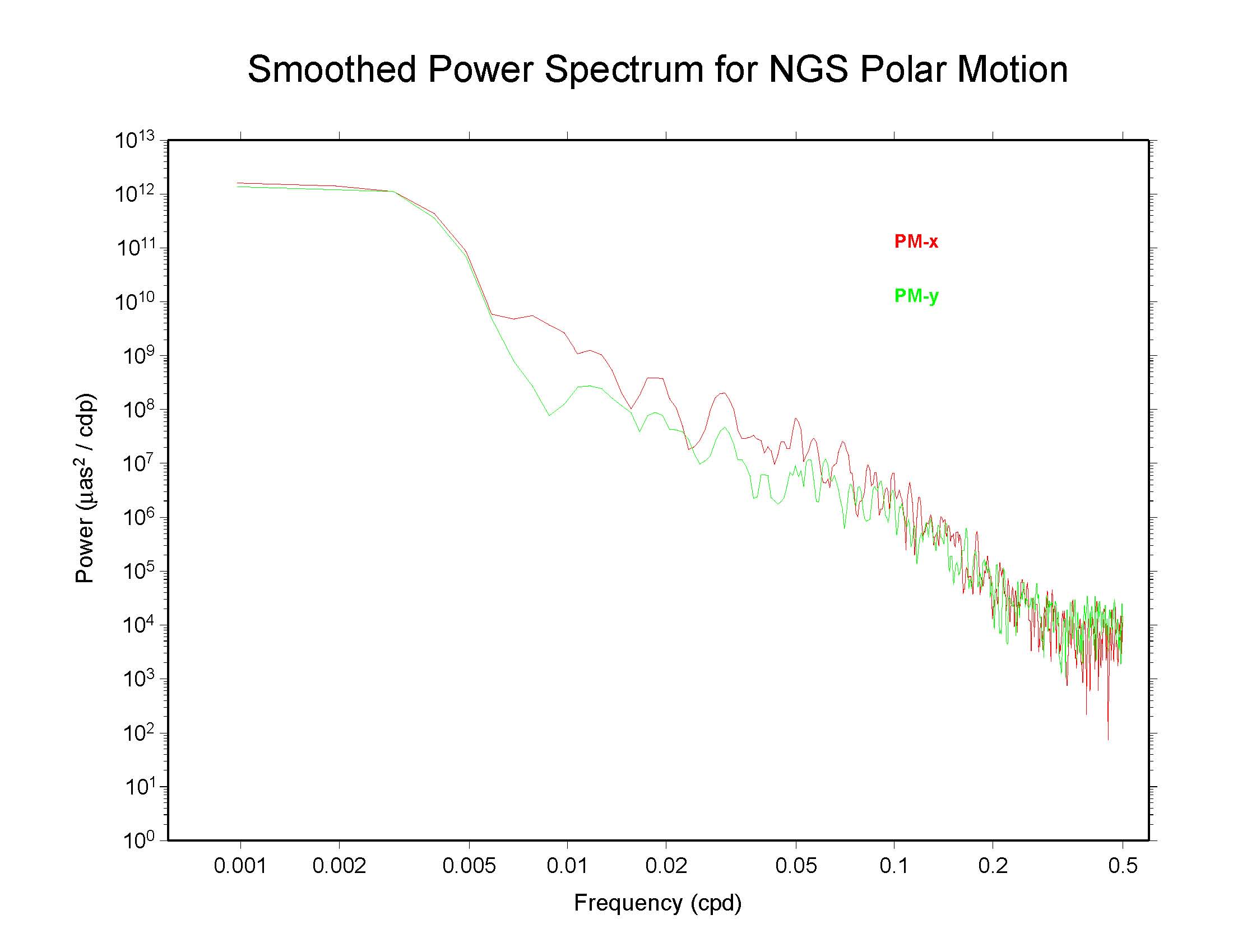
NGS is definitely noise-dominated at the highest frequencies.
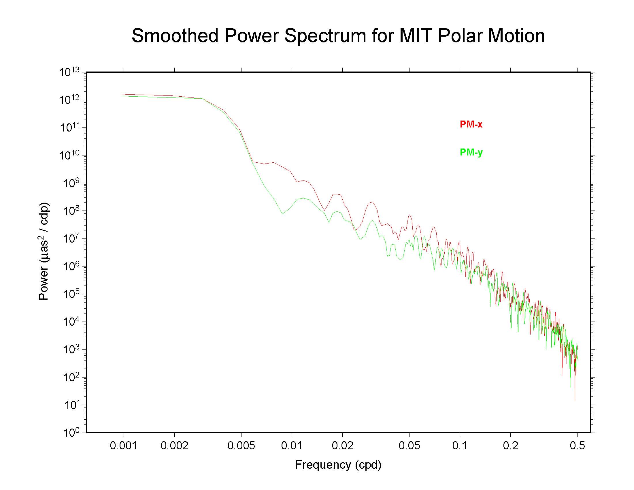
CODE and MIT show strong smoothing at the highest frequencies. It is
probably the effect of these solutions, especially, that causes the
IGS combined series to appear smoothed.
Day-boundary Discontinuities in Polar Motion Series
The apparent smoothing in the CODE and MIT polar motion spectra is probably due to forcing continuity between adjacent days in the estimation of daily offsets and rates. In fact, there are no independent polar motion rates in either case. (MIT has discontinued this practice is in now estimating daily independent midday ERP offsets and rates; see this message from Tom Herring.) Consequently, the IGS combination inherits the smoothing applied in those AC solutions that do not adjust daily independent estimates.
To verify this conjecture, the discontinuities in the polar motion time series have been computed and plotted. The differences at each midnight epoch were found by [PM(day2) - (0.5*PMrate(day2))] - [PM(day1) + (0.5*PMrate(day1))] for the two successive days day1 and day2.
IGS —
http://www.ngs.noaa.gov/igsacc/erp/igs00p03-dpm.ps
CODE —
http://www.ngs.noaa.gov/igsacc/erp/code-dpm.ps
EMR —
http://www.ngs.noaa.gov/igsacc/erp/emr-dpm.ps
ESA —
http://www.ngs.noaa.gov/igsacc/erp/esa-dpm.ps
GFZ —
http://www.ngs.noaa.gov/igsacc/erp/gfz-dpm.ps
JPL —
http://www.ngs.noaa.gov/igsacc/erp/jpl-dpm.ps
MIT —
http://www.ngs.noaa.gov/igsacc/erp/mit-dpm.ps
NGS —
http://www.ngs.noaa.gov/igsacc/erp/ngs-dpm.ps
SIO —
http://www.ngs.noaa.gov/igsacc/erp/sio-dpm.ps
The CODE and ESA polar motion series show discontinuities only at the week boundaries, not each day, confirming the imposition of continuity conditions in both analyses. (Note that for those ACs reporting 9 ERP values each week, the 7 unique middle values have been used here.) The apparent absence of any obvious smoothing in the ESA spectra could be a consequence of greater high-frequency noise masking the effect of the continuity smoothing. The MIT discontinuities were small for most of the period but have increased in the most recent results with the removal of their continuity constraint at the beginning of 2007. (The MIT processing strategy varied in this respect during 2007; see this message.) The situation with SIO is reversed, with a reasonable level of discontinuities initially but continuity constraints were obviously applied starting at the beginning of 2006. Again, high-frequency noise could mask the effect of smoothing in the SIO spectra.
The EMR, GFZ, JPL, and NGS polar motion series do not show any evidence of (strong) day-to-day continuity constraints, although the most recent GFZ scatter is smaller than earlier. However, please note this information from Gerd Gendt. The general improvement in the NGS analysis results over the period is also apparent. For some unknown reason, the scatter in the IGS discontinuities, which are generally very small, increased in late 2007, especially in the PM-y component.
Spectra of Polar Motion Discontinuities at Day Boundaries
Also apparent from the discontinuity plots is the fact that the distributions of polar motion differences are not very random and certainly do not obey white noise statistics. Clear systematic variations can be seen. This is an indication, among other things, of longer-term biases in the polar motion rate estimates. The EMR, GFZ, JPL, and NGS results are good examples of such effects.
Spectra of the day-boundary differences in polar motion are plotted below for these four ACs and the IGS combination. In each case a boxcar filter has been used to smooth across each three adjacent frequencies. The other ACs are not included due to the strong continuity constraints (CODE, ESA, MIT, and SIO) or because of changes in procedures (MIT and SIO).
IGS —
http://www.ngs.noaa.gov/igsacc/erp/igs00p03-dpmsp3.ps
EMR —
http://www.ngs.noaa.gov/igsacc/erp/emr-dpmsp3.ps
GFZ —
http://www.ngs.noaa.gov/igsacc/erp/gfz-dpmsp3.ps
JPL —
http://www.ngs.noaa.gov/igsacc/erp/jpl-dpmsp3.ps
NGS —
http://www.ngs.noaa.gov/igsacc/erp/ngs-dpmsp3.ps
The spectra for the differences of the IGS combination are not very informative because of the influence of contrained AC solutions that were included. EMR, GFZ, and JPL all show prominent peaks with fortnightly periods, and EMR and GFZ also seem to possess peaks near 7 and 9 day periods. Any peaks in the NGS spectra are less apparent.
The table below summarizes the periods for the main peaks near fortnightly, 9-d, and 7-d periods for EMR, GFZ, and JPL.
| Spectral Peaks in PM Differences for ACs without Continuity Constraints | |||
| AC | 14 d | 9 d | 7 d |
| EMR PM-x ± |
14.2 0.2 |
9.35 0.09 |
7.18 0.05 |
| EMR PM-y ± |
14.1 0.2 |
9.6 & 9.0 0.1 |
7.16 0.05 |
| GFZ PM-x ± |
14.2 0.2 |
9.4 0.1 |
7.21 0.05 |
| GFZ PM-y ± |
14.2 0.2 |
9.6 & 8.9 0.1 |
7.14 0.05 |
| JPL PM-x ± |
14.2 0.2 |
9.4 0.1 |
7.23 0.05 |
| JPL PM-y ± |
14.2 0.2 |
9.2 0.1 |
7.26 0.05 |
EMR, GFZ, and JPL all have prominent fortnightly peaks for both polar motion components at 14.2 d with a resolution of about ± 0.2 d. The second-largest peaks for EMR and JPL are near 9.4 d, but the PM-y component is split for EMR. This same peak is third-largest for GFZ and also split for the PM-y component. There is a weekly peak at 7.2 d but it is weak for JPL.
Possible Sources of Spectral Peaks in PM Differences
Kouba (2003) showed that errors in the a priori analysis model for subdaily Earth orientation variations can alias against the IGS 24-hr processing interval to create longer-period signals in the polar motion rate estimates. (The pole offsets are not materially affected due to near complete averaging over 24 hr.) The alias periods for the eight main subdaily tides are shown in the table below; negative periods indicate retrograde variations.
| Alias Peaks due to Errors in Subdaily EOP Model | ||
| Tide wave | Period (hr) | Alias period (d) |
| M2 | -12.42 | 14.75 |
| S2 | -12.00 | infinity |
| N2 | -12.66 | 9.62 |
| K2 | -11.97 | -181.32 |
| K1 | 23.94 | 368.23 |
| O1 | 25.82 | -14.19 |
| P1 | 24.07 | -364.64 |
| Q1 | 26.87 | -9.37 |
As pointed out by Jan Kouba in this message the observed spectral peak at 14.2 d almost certainly corresponds to the aliased O1 ocean tide error in the subdaily models used by EMR, GFZ, and JPL. There is also some possibility that the observed peaks near 9.4 and 9.6 d could be caused by aliased errors of Q1 and N2 tides, respectively, but a similar explanation is not evident for the weekly peak at 7.2 d. It cannot be overstated how useful it would be to have current analysis summaries for all the IGS ACs to check into such questions.
An alternative explanation is that the observed peaks might be due to second-degree zonal tide signatures in polar motion via ocean excitation; see Gross et al. (1996) and Gross et al. (1997). In this case the expected tidal periods are shown in the table below.
| Zonal Tidal Polar Motion Periods | ||
| Tide wave | Period (d) | Fundamental arguments |
| l, l', F, D, omega | ||
| M9 | 9.12 | 1, 0, 2, 0, 1 |
| M9' | 9.13 | 1, 0, 2, 0, 2 |
| Mf | 13.63 | 0, 0, 2, 0, 1 |
| Mf' | 13.66 | 0, 0, 2, 0, 2 |
| Mm | 27.55 | 1, 0, 0, 0, 0 |
| Ssa | 182.62 | 0, 0, 2, -2, 2 |
| Sa | 365.26 | 0, 1, 0, 0, 0 |
The fortnightly zonal peaks, while small, have been detected in polar motion time series; see the Gross et al. references above. However, these variations in the pole offsets are greatly attenuated in the polar motion differences computed here, which are mostly sensitive to rate errors. Since the fortnightly, especially, and 9-d peaks expected for the zonal tides do not match the observed IGS peaks, this argues against a direct geophysical origin for the latter. An explanation for the small weekly peak remains elusive, although it could conceivably come from unremoved atmospheric excitation or might be related in some way to the daily IGS sampling.
Consequences and Issues to Consider
There are numerous issues raised by those analysis procedures that do not provide fully independent daily ERP estimates. Fundamentally, the ERP information types among the ACs are not internally the same quantities and a meaningful combination is not strictly possible. Not only does a continuity constraint smooth the resulting high-frequency ERP estimates, but it is also a very strange type of phase filter that passes Nyquist-frequency signals with cosine phase aligned to the day boundaries but completely attenuates the same frequencies when shifted by 90 degrees. So the high-frequency signal content is substantially modified as well as smoothed.
This point can be visualized in the following way. Consider a cosinusoid with period equal to the Nyquist period, 2 days in the case of the daily ERP estimates. Then when the phase of the cosine is aligned with the day boundaries (at midnight epochs), the situation illustrated below applies:
Case 1.  Cosine signal with Period = 2d, phase =  0 deg

      |                 |                  |
 +1   |                 C                  |
      |              *  |  *               |
      |            *    |     *            |
      |           *     |      *           |
      |          *      |       *          |
      |         *       |        *         |
 -----+--------O--------+---------O--------+-----
      |       *         |          *       |
      |      *          |           *      |
      |     *           |            *     |
 *    |    *            |             *    |    *
   *  |  *              |               *  |  *
 -1   C                 |                  C
      |                 |                  |
             Day 1             Day 2


 Continuous offset values (C):

   C(Day1,t=0)  = -1.0
   C(Day1,t=24) =  1.0
   C(Day2,t=0)  =  1.0
   C(Day2,t=24) = -1.0

 Offset + rate values (O):

   O(Day1,t=12) = 0.0
   rate(Day1,t=12) = 2/24 = 0.08333
   O(Day2,t=12) = 0.0
   rate(Day2,t=12) = -2/24 = -0.08333

 ==> both methods give exactly same fits;
     attenuation of signal by continuous method = 0%
The two types of parameterization, while seemingly different, actually are equivalent; they fit the cosine wave in the same way. However, this circumstance is not generally true. Consider now the same cosine but with its phase shifted by 90 degrees:
Case 2.  Cosine signal with Period = 2d, phase = -90 deg

      |                 |                  |
 +1   |        *        |                  |
      |     *     *     |                  |
      .+++*++++O++++*+++.                  |   *
      |  *           *  |                  |  *
      | *             * |                  | *
      |*               *|                  |*
 ---==C=================C==================C==---
     *|                 |*                *|
    * |                 | *              * |
   *  |                 |  *            *  |
  *   |                 .+++*++++O+++++*+++.
      |                 |     *     *      |
 -1   |                 |        *         |
      |                 |                  |
             Day 1             Day 2


 Continuous offset values (==C==):

   C(Day1,t=0)  = 0.0
   C(Day1,t=24) = 0.0
   C(Day2,t=0)  = 0.0
   C(Day2,t=24) = 0.0

 Offset + rate values (++O++):
   O(Day1,t=12) = 0.64
   rate(Day1,t=12) = 0.0
   O(Day2,t=12) = -0.64
   rate(Day2,t=12) = 0.0

 ==> two methods give totally different fits;
     attenuation of signal by continuous method = 100%
In this case the two parameterizations give strikingly different results. The independent daily offset + rate approach is as sensitive to this input phase as for any others, whereas the continuous linear segment (CLS) parameterization totally attenuates the input signal. It is for this reason that the CLS method yields a power spectrum for the polar motion estimates that has the appearance of being smoothed at the highest frequencies, as shown in the plots above (compare CODE to GFZ, for instance). The power at the Nyquist limit is reduced by nearly an order of magnitude for the CLS method compared to the daily independent offset + rate parameterization. The smoothing and signal distortion effects extend to roughly 5 segment lengths, judging empirically from the spectrum plots. Thus, while the CLS method is sometimes claimed to be an "efficient" style of parameterization, it most definitely is not.
It is important to note that the CLS attenutation of certain signals near the Nyquist frequency creates an opportunity for those geophysical variations to alias into other parameters included in the solution. For instance, CLS parameterization of daily ERP variations will force some unwanted ERP effects near 2-day periods into spurious rotations of the satellite orbit frame and/or the terrestrial frame. Similarly, CLS tropospheric delay estimation will alias some atmospheric error into mainly station height estimates, especially if high-rate (dynamic) positioning is attempted. As a counter-measure, additional continuity constraints or lengthened parameterization intervals (e.g., multi-day orbit arcs) are often used for the other parameters. Naturally, these tactics limit the temporal resolution of all parameters, while simultaneously smoothing them and distorting their signal content.
In addition to these important considerations of spectral and signal content, there are other practical considerations. In particular, the ERP series from the non-compliant ACs are not consistent with the longstanding request from the IERS for 24-hr integrations, which consequently causes inherent over-smoothing in the resulting IERS polar motion combinations because of the high weight enjoyed by the IGS. Simple time series combinations and analyses are greatly complicated by the fact that CLS parameterization causes all the parameter estimates to be much more highly correlated with one another than with offset or offset + rate approaches. In most published work, the correlations are ignored, which can lead to invalid conclusions.
Equally important, the resulting series are less useful for studies of the high-frequency excitation of geophysical processes, such as Earth rotations (see next section, for instance), and for diagnositic studies of the type shown here. In CLS parameterization, constraints are applied to the system of GPS observations equations that are totally unnecessary and invariably inconsistent with the data at some level. Nothing is gained in the process and the undesirable side-effects cannot be easily quantified nor can they be removed. As originally outlined at the IGS 1996 Analysis Workshop held at Silver Spring, MD, USA, the estimation of midday daily offsets and rates provides effectively twice-daily ERP samples with some measure of subdaily resolution. The mechanisms for setting up and reporting ERP parameterization were agreed at the IGS 1998 Workshop held in Darmstadt, Germany. For tropospheric delay estimation, simple segmented offsets at regular intervals (or Kalman filter modeling) is much preferred over continuous linear segments. For standard GPS data processing, tropospheric offsets need not apply for intervals longer than 1 hour, although much higher temporal resolution can be achieved with Kalman filtering.
Given that the precision (probably around 30 µas) and accuracy of the IGS polar motion estimates are much better than from any other observing technique, it is important for us to take the utmost care not to introduce spurious errors and other avoidable effects, such as a priori smoothing and CLS distortion. Many of the proposals discussed at the IERS Monterey workshop in December 2007 would exacerbate the problems illustrated here by sanctioning the use of non-independent parameter estimates in SINEX. That misguided idea would clearly degrade IERS and IGS products.
Subdaily Polar Motion Variability
One of the main reasons to examine the high-frequency polar motion spectra is to estimate how large subdaily variations might be, apart from the oceanic tidal effects. With the smoothed and distorted spectra it is not possible to make such an assessment. So, using only the GFZ polar motion spectra, a fit has been made for the power spectral indices over the frequency range from 0.1 to 0.5 cpd to get:
       Px(f) = (48.1063 µas2/cpd) * (f/cpd)-4.5491
       Py(f) = (64.2146 µas2/cpd) * (f/cpd)-4.0979
If one assumes that these power-laws apply also for freq > 0.5 cpd and then integrate over freq = 1 -> infinity, one obtains:
       Varx(1->inf) = 13.5545 µas2
       Vary(1->inf) = 20.7284 µas2
Even if the precision of IGS polar motion estimates for 1-d integrations reaches a level around 30 µas or so, it remains that there are almost certainly systematic errors due to data mismodeling and other effects, as noted above. Those errors could be worse near tidal lines. In any case, it seems unreasonable to think that any background polar motion continuum power could be observable over the subdaily regime using present technologies. A better approach than a broadband parameterization would probably be to estimate specific tidal (or other) waves with known frequencies, if there is an interest to examine this part of the spectrum in greater detail.
Measures to Mitigate Undesired Smoothing
It is important to resolve how the IGS products should be formed. The present procedure mixes dissimilar estimates. If all ACs can modify their processing to provide the requested daily offsets and rates (or equivalent), this would seem to be optimal. Otherwise, it is better to use only the subset of compliant solutions for the time being.
Starting with GPS week 1460, it is proposed to exclude the ERPs submitted by CODE and ESA from the IGS combined ERPs, assuming that SIO will remove (or deweight) their ERP continuity constraint. If ESA can also remove its constraints by week 1460 or whenever their new software is implemented operationally, that would be greatly appreciated.
For the IGS reprocessing effort, which begins with week 1459 and will work backwards in time, I presume that PDR estimates its ERPs the same way as CODE and therefore theirs should also not be used. Can all other ACs affirm that they will apply no (or weak) ERP continuity constraints?
I welcome discussion of this matter.
| Send comments to Jim Ray | (updated 05 February 2008) |