 |
|
|
| |
|
|
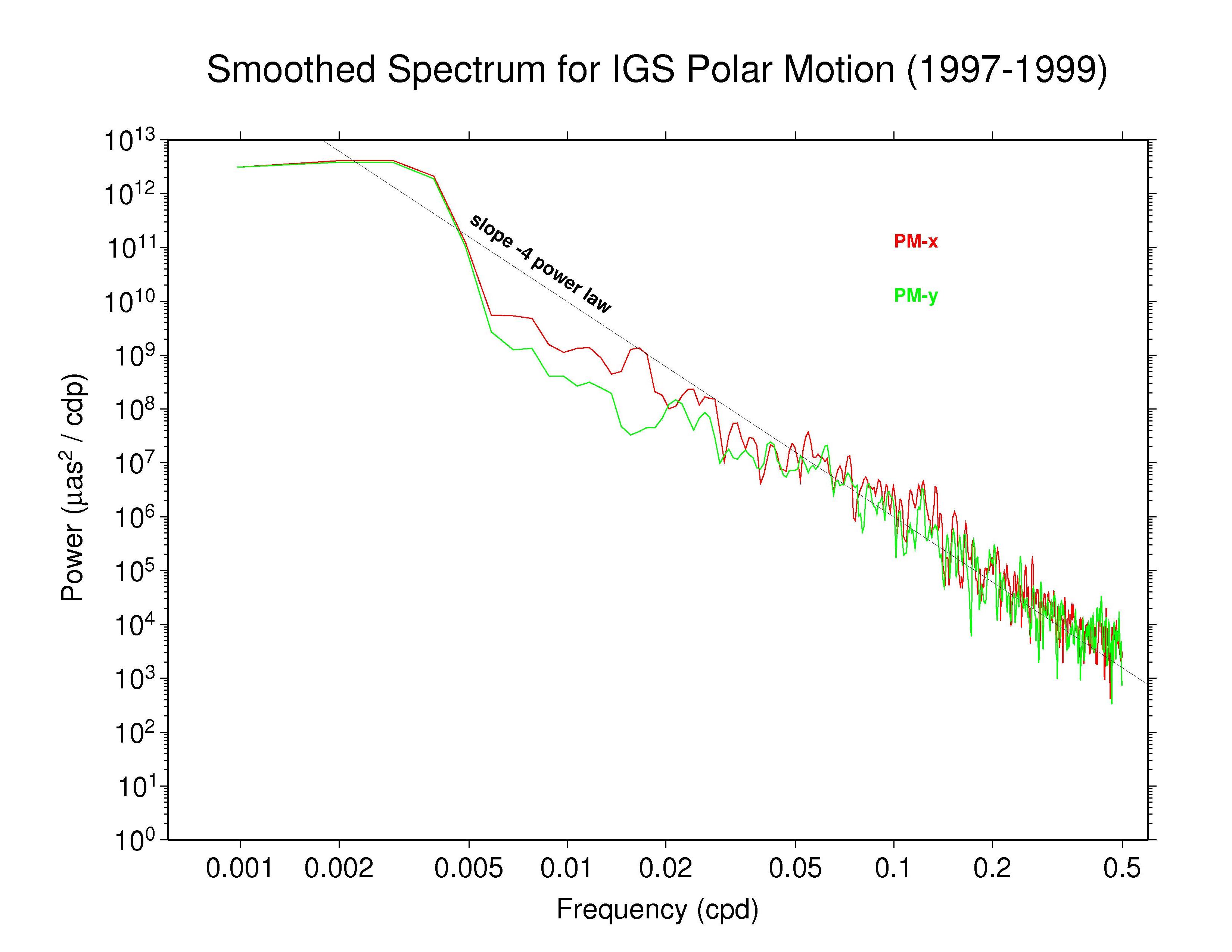
Power spectra have been generated and are plotted below for the polar motion time series computed from the IGS submission for ITRF2008. The IGS submission consists of weekly SINEX files produced by Remi Ferland (NRCanada) by combining Earth rotation results (together with the associated terrestrial frames) from 7 of the 11 Analysis Centers (ACs) participating in the IGS Reprocessing Campaign #1 (repro1) for the period 1997-2007 (inclusive) plus operational solutions from seven of the regular eight Final ACs for the period 2008-2009.5. (The AC solutions used were those available in time to satisfy the ITRF2008 delivery deadline. Additional ACs will be included in the final repro1 combination.) These weekly TRF+EOP solutions, in SINEX format, have been accumulated in a long-term stacking procedure by Zuheir Altamimi (IGN) to generate a consistent linear reference frame and associated EOP time series. It is necessary to identify each position and/or velocity discontinuity in the time series of each IGS station in order to properly model such events as discrete breaks, a process that has been done by Remi and iterated by Zuheir.
In order to gauge the extent to which results have evolved with time, the full span of 12.5 years has been broken into four separate, non-overlapping segments: 1997-1999, 2000-2002, 2003-2005, and 2006-2009.5. The results presented here can be compared with a previous study of IGS operational polar motion results by Ray (2008), which covered the 1024 days from MJD 53412.5 (week 1309_5 or 11 Feb 2005) to 54435.5 (week 1455_6 or 01 Dec 2007). The consequences of polar motion smoothing by imposition of day-to-day continuity constraints was discussed in considerable detail there. An analysis of reprocessed polar motion results for the period 2005-2007, including individual AC results as well as the IGS combination for that span, is available at Ray (2009). That study includes some AC solutions not available for the ITRF2008 submission.
For the plots below a smoothing across each three adjacent frequencies has been applied with a sliding boxcar filter to make the appearance less noisy (but unsmoothed plots are also available and are not substantially different). In each case, the smoothed spectrum for the PM-x component of polar motion is shown as the red curve and the PM-y component is shown in green.
Most continuous geophysical processes and most physical noise processes
possess power spectra that decrease as the frequency raised to some
characteristic negative power ("spectral index"). The spectra are usually
"reddish" in the sense of having more power at the lower frequencies
(i.e., longer periods). For reference, a power law with spectral index
of -4 is drawn on each plot (not a fit). This corresponds to the
behavior of an integrated random walk (in phase) noise process, that is,
a doubly integrated white noise process.
  IGS (1997-1999) —
ps file IGS (1997-1999) —
ps file
|
 IGS (2000-2002) —
ps file IGS (2000-2002) —
ps file
|
 IGS (2003-2005) —
ps file IGS (2003-2005) —
ps file
|
 IGS (2006-2009.5) —
ps file IGS (2006-2009.5) —
ps file
|
It is important to note that not all ACs contribute solutions equally
for all periods. This is because the IGS ITRF2008 submission was
formed from a "snapshot" of the reprocessed AC solutions available at
the time of the ITRF deadline. Later, all repro1 solutions will be
used for a final combination series; see the
IGS Reprocessing Campaign #1 (repro1) website. For the results
presented here, the array of ACs contributing polar motion solutions
can be summarized as:
The AC names above ending with "1" indicate reprocessed solutions whereas other names indicate regular operational IGS Final solutions. The analysis here combines the 2006-2007 and 2008-2009.5 periods into a single span.
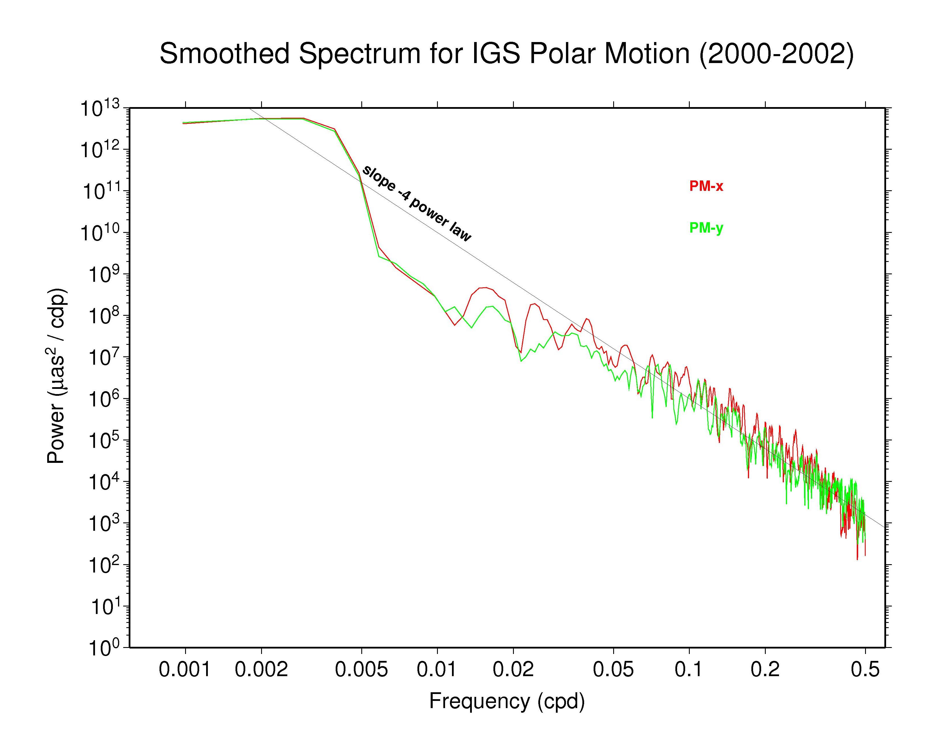
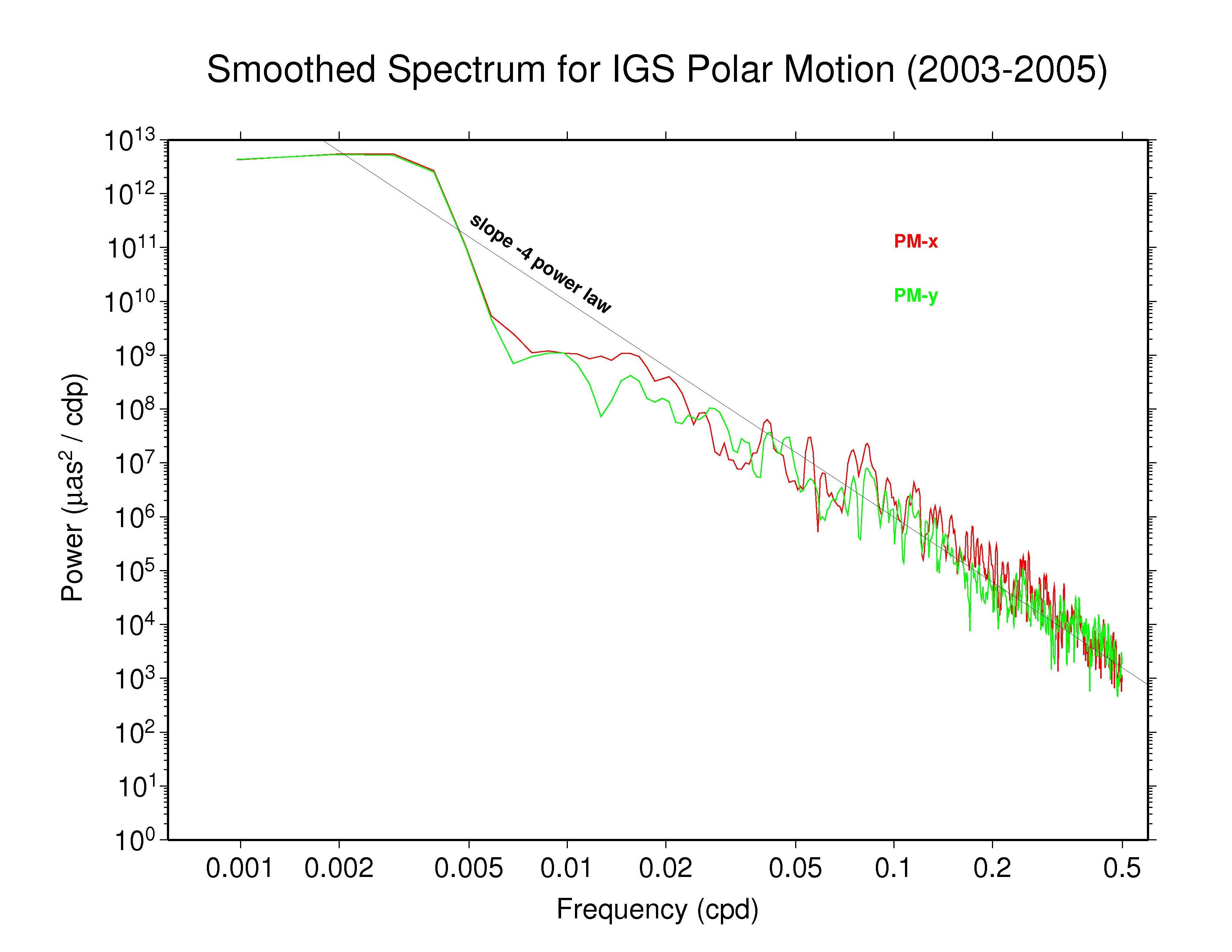
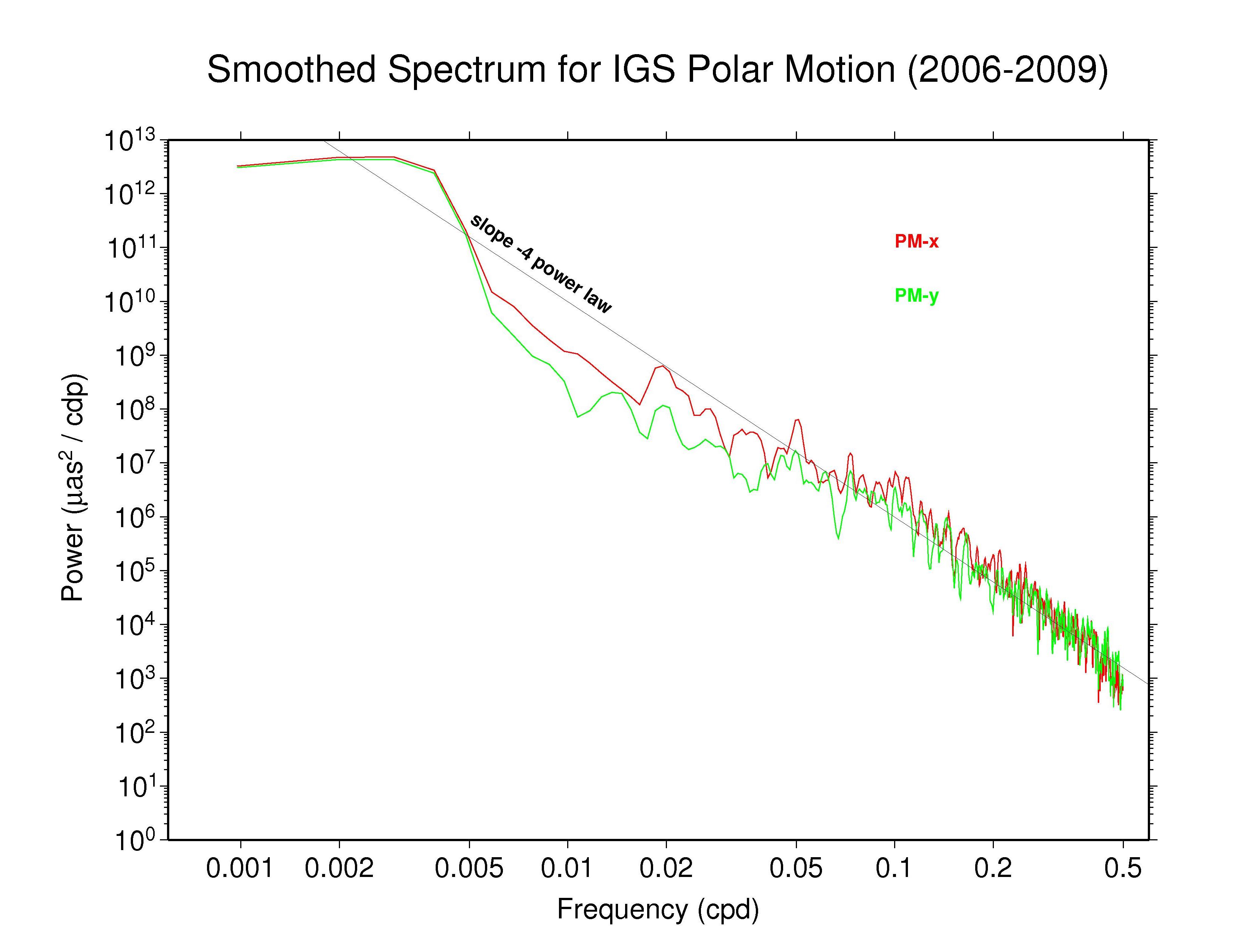
The IGS spectra for all four periods are substantially similar. Both polar motion components have nearly equal power at annual periods and both drop in power faster than a slope -4 power law during inter-seasonal intervals. For periods shorter than about 20 days, both components follow rather closely a slope -4 power law, with PM-x generally having somewhat greater power than PM-y. Approaching the Nyquist limit of 2 d, the character of the spectra is more distinct for the different spans of data. In the results from the earliest data, a high-frequency noise floor is apparent, but this vanishes after about 2000. Instead, starting around 2003 it appears that some effective smoothing may attenuate the highest-frequency power. Smoothing of this type was seen in earlier IGS operational polar motion series (Ray, 2008) where it was argued that the effect was a consequence of imposing day-to-day continuity (or similar) constraints by some ACs. The situation with this new series should be different since ACs were asked to avoid applying any over-constraints in their solutions, else their polar motion contributions were excluded from the combination. For a characterization of the individual AC reprocessed polar motion series for the period 2005-2007, please see Ray (2009).
The underlying cause for the apparent smoothing in the IGS combined polar
motion results since about 2003 needs further investigation. It could
indicate, for instance, that the reported SINEX ERP constraints are not
being fully removed or that some ACs have unreported constraints that are
not entirely negligible. The varying high-frequency behaviors seen above
could reflect either the evolution of the GPS data/network quality or
changes in the mix of AC solution used (see tabulation above).
IGS Polar Motion Formal Errors
To see if the apparently larger high-frequency noise seen above in the
IGS reprocessed polar motion power spectra before 2000 is reflected in
the formal errors of the estimates, those are plotted below. In forming
each weekly SINEX combination, Remi rescales the input AC covariance
matrices based on their agreement with the IGS05 reference frame. To
form his long-term linear stacking of these weekly solutions, Zuheir
makes another adjustment of the IGS combined covariances to ensure
consistency with the VLBI solutions provided by the IVS. The polar
motion formal errors shown below are the result of both rescalings.
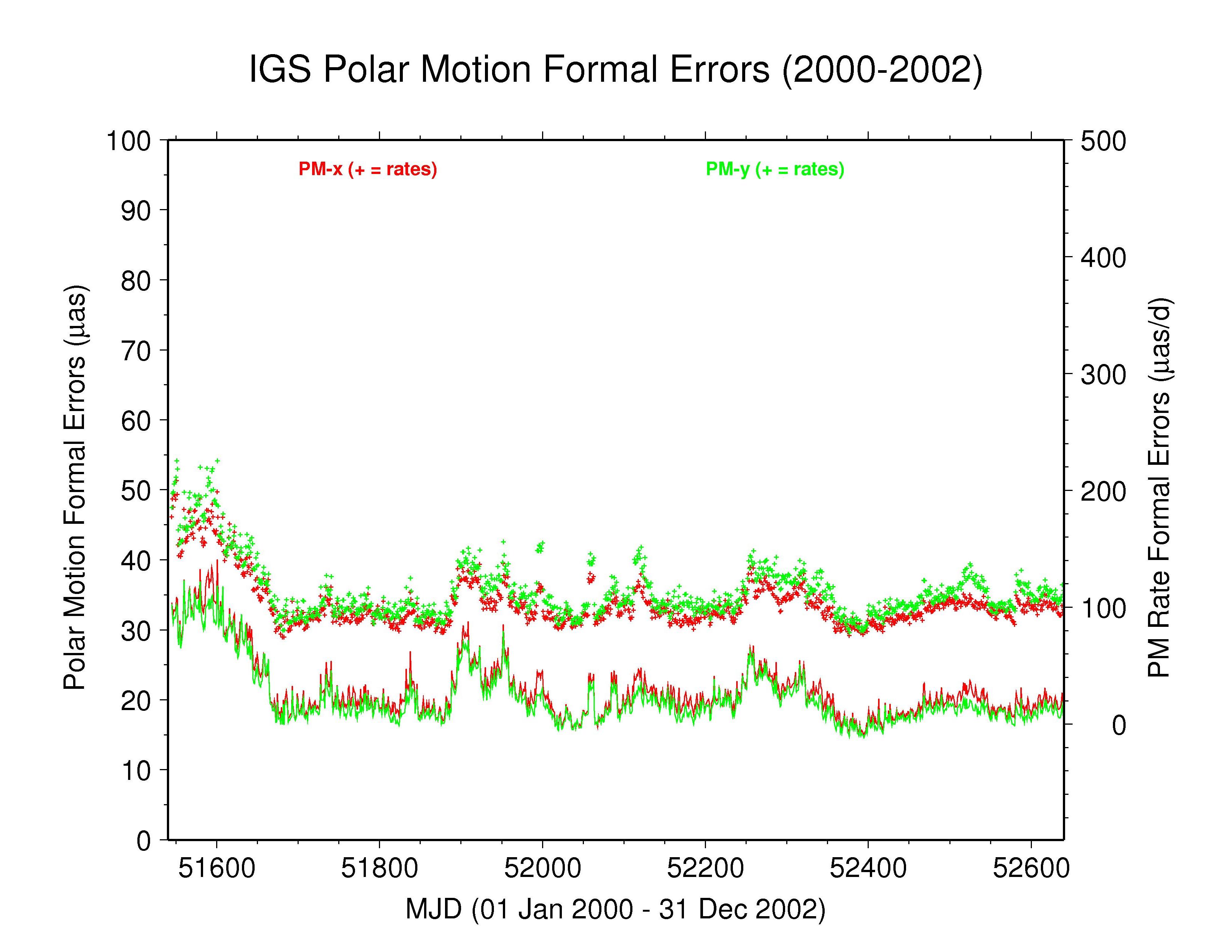
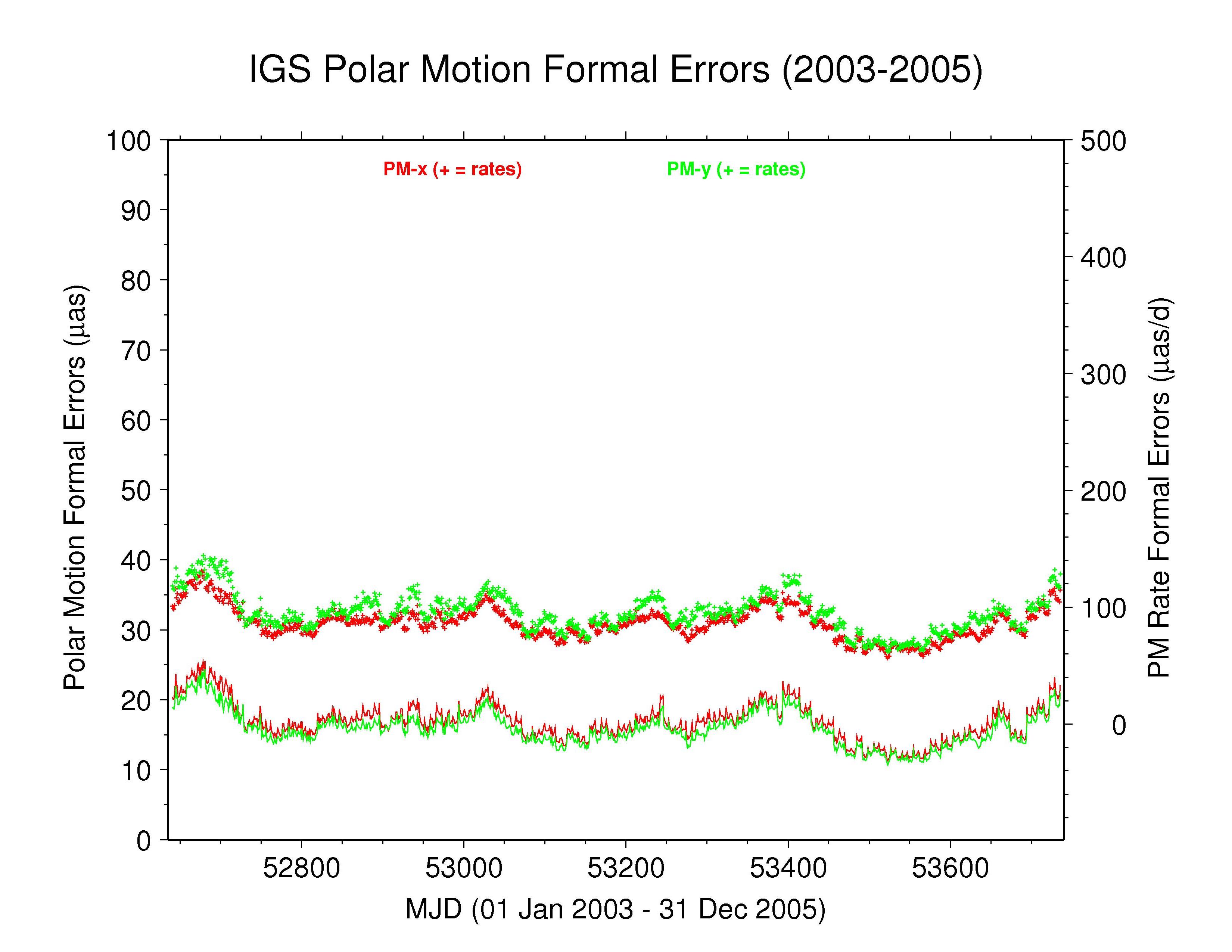
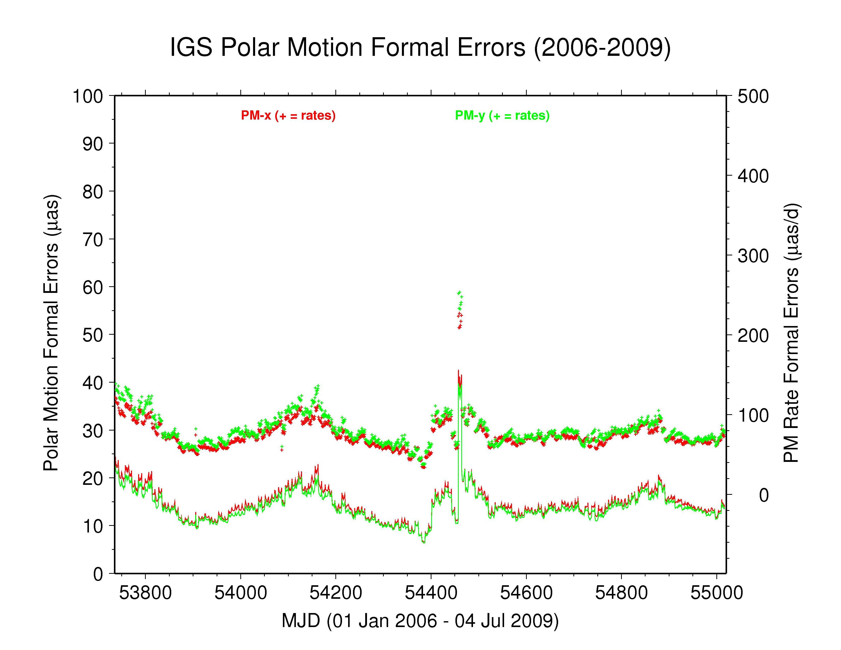
PM-x component formal errors are shown in red and PM-y component formal
errors shown in green; the PM offset errors (left scale) are connected by
lines while the PM rate errors (right scale) are crosses.
 IGS (1997-1999) —
ps file IGS (1997-1999) —
ps file
|
 IGS (2000-2002) —
ps file IGS (2000-2002) —
ps file
|
 IGS (2003-2005) —
ps file IGS (2003-2005) —
ps file
|
 IGS (2006-2009.5) —
ps file IGS (2006-2009.5) —
ps file
|
The IGS polar motion formal errors are relatively stable after late April 2000 (after about MJD 51663.5), at the level of about 20 µas for offsets and about 100 µas/d for rates. The rate errors closely parallel the offset errors. There is an overall annual modulation in the the later formal errors, except for period in late 2007 of disturbed errors. GPS week 1459 (23-29 Dec 2007) has anomalously large formal errors, which must represent some problem in the combination of AC solutions, or the solutions themselves, for that week. The PM-x offset formal errors are generally a bit larger than for PM-y, while the reverse is true for the rates. There is a strong, but small, weekly modulation in both offset and rate components. Spectra (not shown) confirm this for the results since 2000 as well as revealing harmonics at 7/2 d and 7/3 d (only for the period since 2003). This is presumably related to the IGS weekly processing cadence and is therefore undoubtedly an analysis artifact contributed by certain ACs. Inspection of the individual AC repro1 polar motion series for the 2005-2007 period reveals no weekly harmonics in the formal errors of EM1, ES1, JP1, NG1, SI1, or UL1. The GF1 and GT1 errors do show such harmonics, however, and perhaps also MI1 to lesser extent. The ES1 errors have an odd drop in power at 7 d while GF1 and GT1 have a similar drop at a slightly longer period.
Unsurpringly, before April 2000, the polar motion formal errors increase steadily the older the data become and the character of the errors differs from the more recent data. Annual modulations are much less evident and the weekly variations seen in later data are not present.
Day-boundary Discontinuities in IGS Polar Motion Series
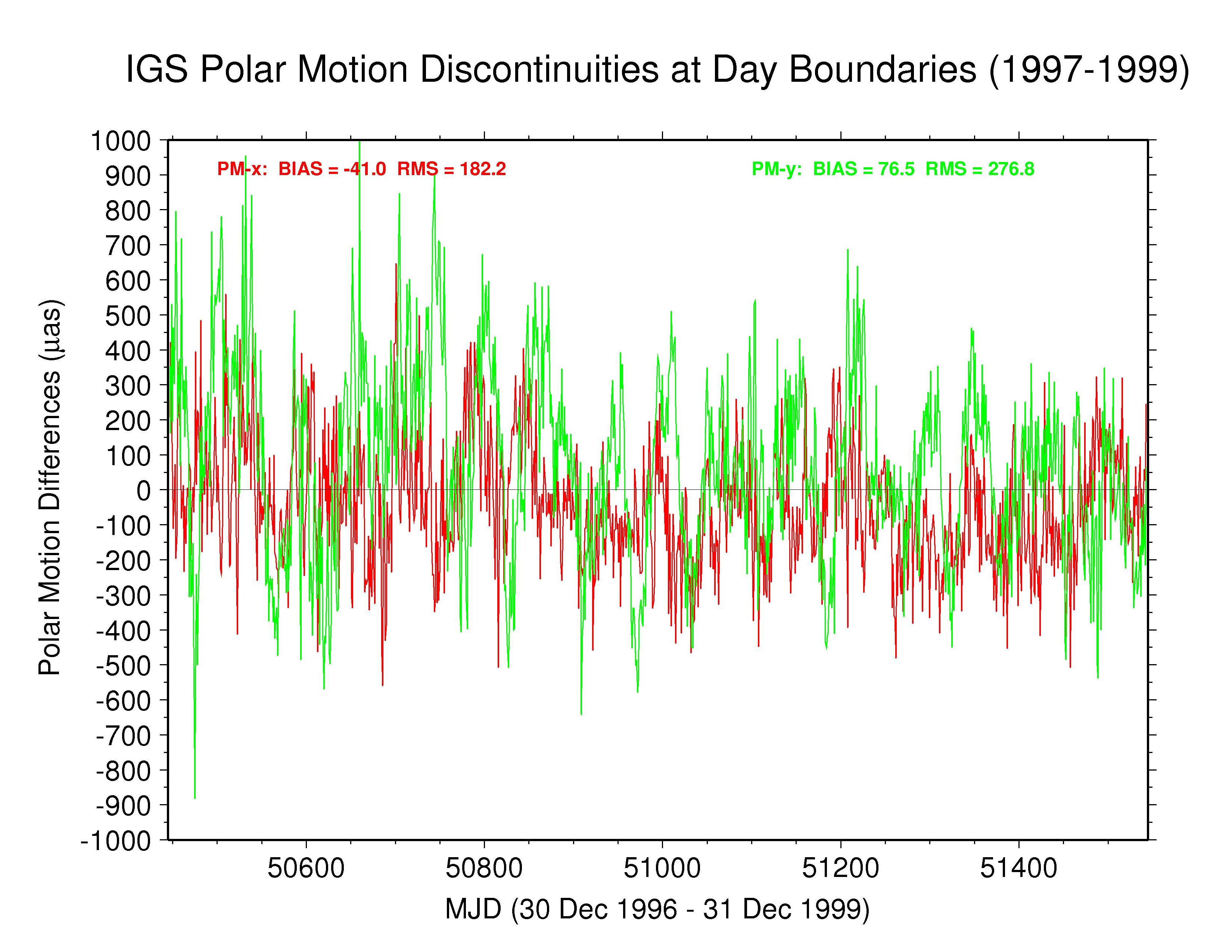
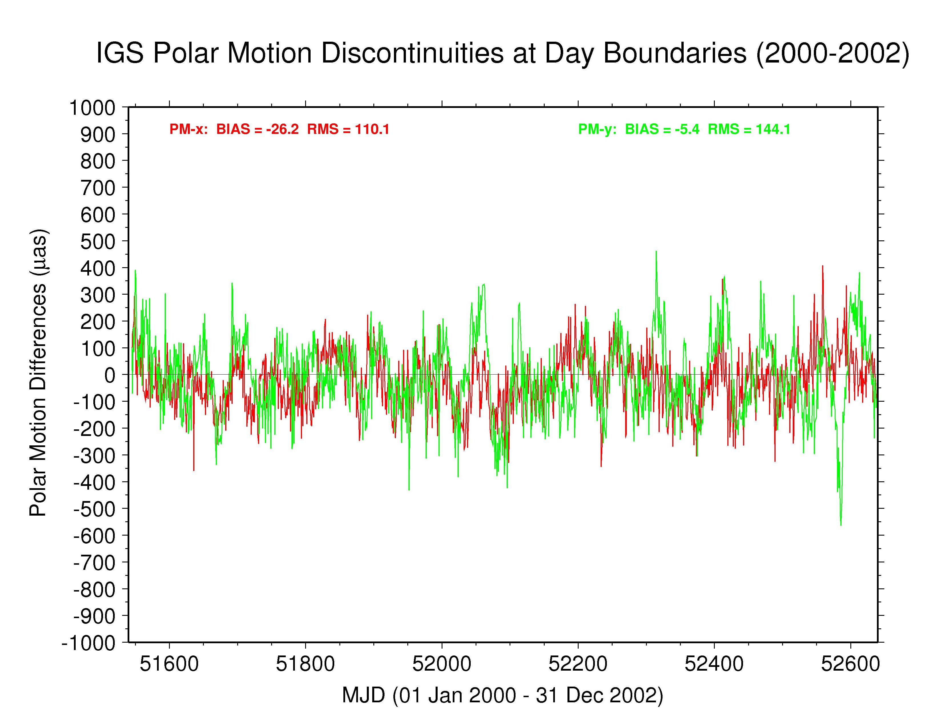
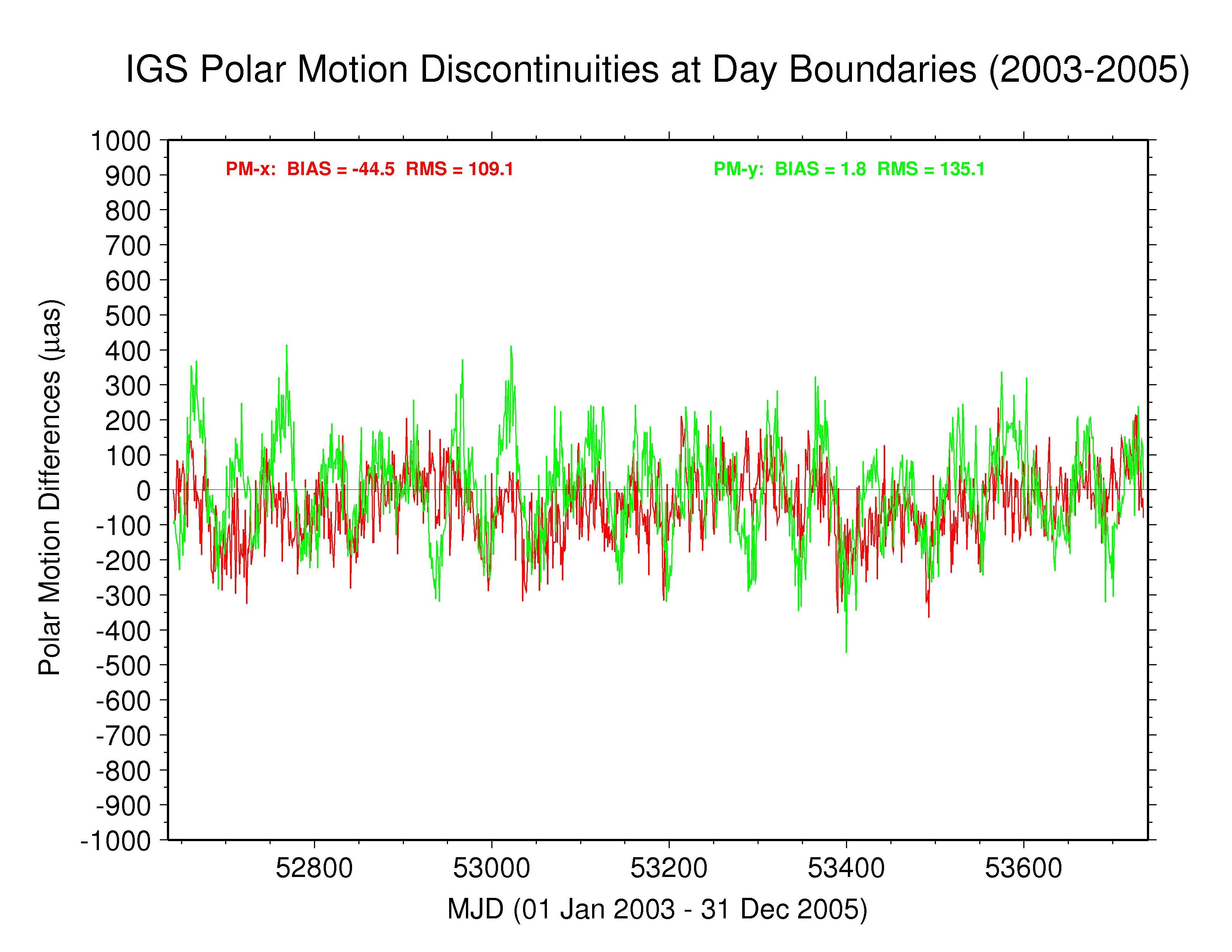
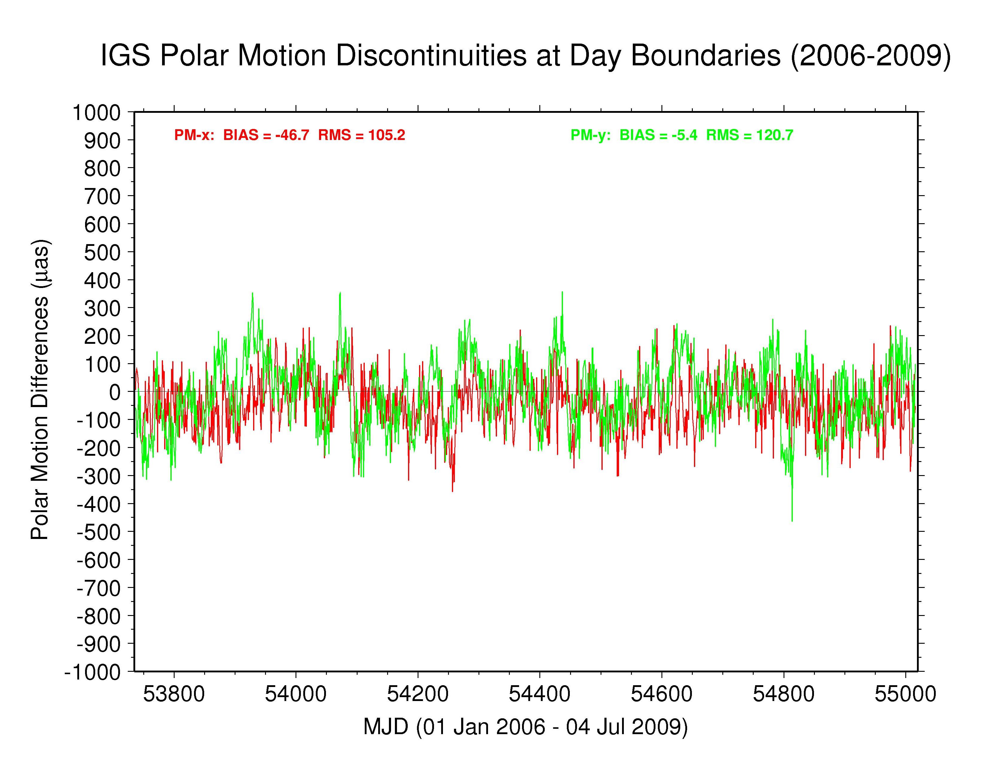
To examine the extent to which continuity conditions have been imposed on the polar motion rate parameters between days and to characterize the performance of the polar motion rate estimates, the discontinuities in the polar motion time series have been computed at day boundaries and plotted below. The differences at each midnight epoch were found by [PM(day2) - (0.5*PMrate(day2))] - [PM(day1) + (0.5*PMrate(day1))] for each successive pair of days, day1 and day2. PM-x component discontinuities are shown in red while PM-y component discontinuities are shown in green. On each plot is also shown the (unweighted) mean bias and RMS for each component.
Note that the variations shown here reflect almost entirely the behavior of the polar motion rate estimates, not the mid-day polar motion offsets. As long as no strong continuity constraint is imposed on the rate estimates, their variations (for whatever reason) probably have minimal impact on the associated mid-day (also mid-arc) polar motion offset estimates. This means that end-users of IGS polar motion results should probably rely more heavily on the offset values and not on the rate values, even for studies of geophysical excitation (that is, polar motion rate-of-change). It is probably more reliable to use polar motion change estimates derived from fits to the offsets (via splines, for instance) than to use the directly estimated polar motion rates for reasons that will be demonstrated in the next section.
Polar motion rate estimates are probably most useful as a probe of
the quality of the AC modeling, especially the modeling of
the satellite orbit dynamics, and the a priori subdaily EOP
model reliability than as accurate measures of Earth dynamics. Since
a pole position offset is sensed in the GNSS modeling as a
global diurnal sinusoidal motion of the terrestrial frame relative
to the satellite frame, any similar type constellation-wide errors
in the orbital frame can alias into the polar motion and polar
motion rate estimates. Satellite methods are completely incapable of
detecting diurnal retrograde motions, which for the Earth correspond
to nutations. Consequently, it is also useful to examine the spectra
of the polar motion discontinuities to see if these reveal information
about data modeling deficiencies (see next section).
 IGS (1997-1999) —
ps file IGS (1997-1999) —
ps file
|
 IGS (2000-2002) —
ps file IGS (2000-2002) —
ps file
|
 IGS (2003-2005) —
ps file IGS (2003-2005) —
ps file
|
 IGS (2006-2009.5) —
ps file IGS (2006-2009.5) —
ps file
|
Consistent with the greater high-frequency noise seen above in the spectra of the earliest IGS polar motion results, the day-boundary discontinuities are considerably more variable before about 2000. Mean bias and RMS values (unweighted) are tabulated below for each span of polar motion discontinuity time series. All the results show clear systematic patterns in the time variations of the polar motion discontinuities.
A significant long-term polar motion rate bias is seen in the IGS PM-x
component. This is the average effect of PM-x rate biases inherited
from the AC solutions by MIT, mainly, and to a lesser extent GTZ, ESA,
and SIO; see Ray (2009). The IGS PM-y
rates are much less biased, on average. As seen also in the prior repro1
analysis of results for 2005-2007, the PM-y rates are significantly more
scattered than the PM-x rates. The higher PM-y rate scatter is probably
related to the appearance of stronger harmonics of the GPS draconitic
year (mainly the 5th and 7th multiples; see below)
in that component for most ACs and the IGS combination.
| Statistics of IGS Day-boundary Polar Motion Discontinuities | |||||
| Interval | PM-x (µas) | PM-y (µas) | # days | ||
| bias | RMS | bias | RMS | ||
| 1997-1999 | -41.0 | 182.2 | 76.5 | 276.8 | 1098 |
| 2000-2002 | -26.2 | 110.1 | -5.4 | 144.1 | 1096 |
| 2003-2005 | -44.5 | 109.1 | 1.8 | 135.1 | 1096 |
| 2006-2009.5 | -46.7 | 105.2 | -5.4 | 120.7 | 1281 |
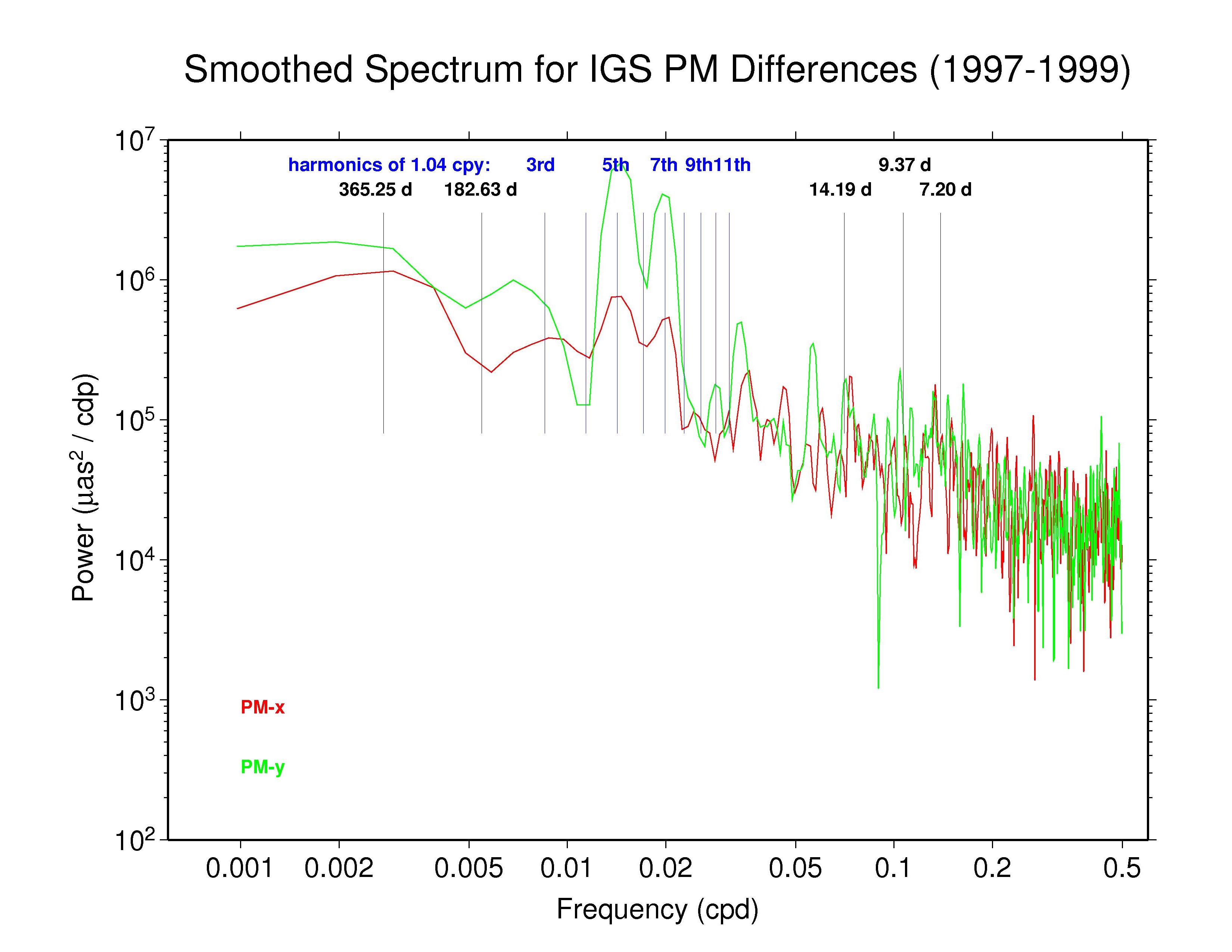
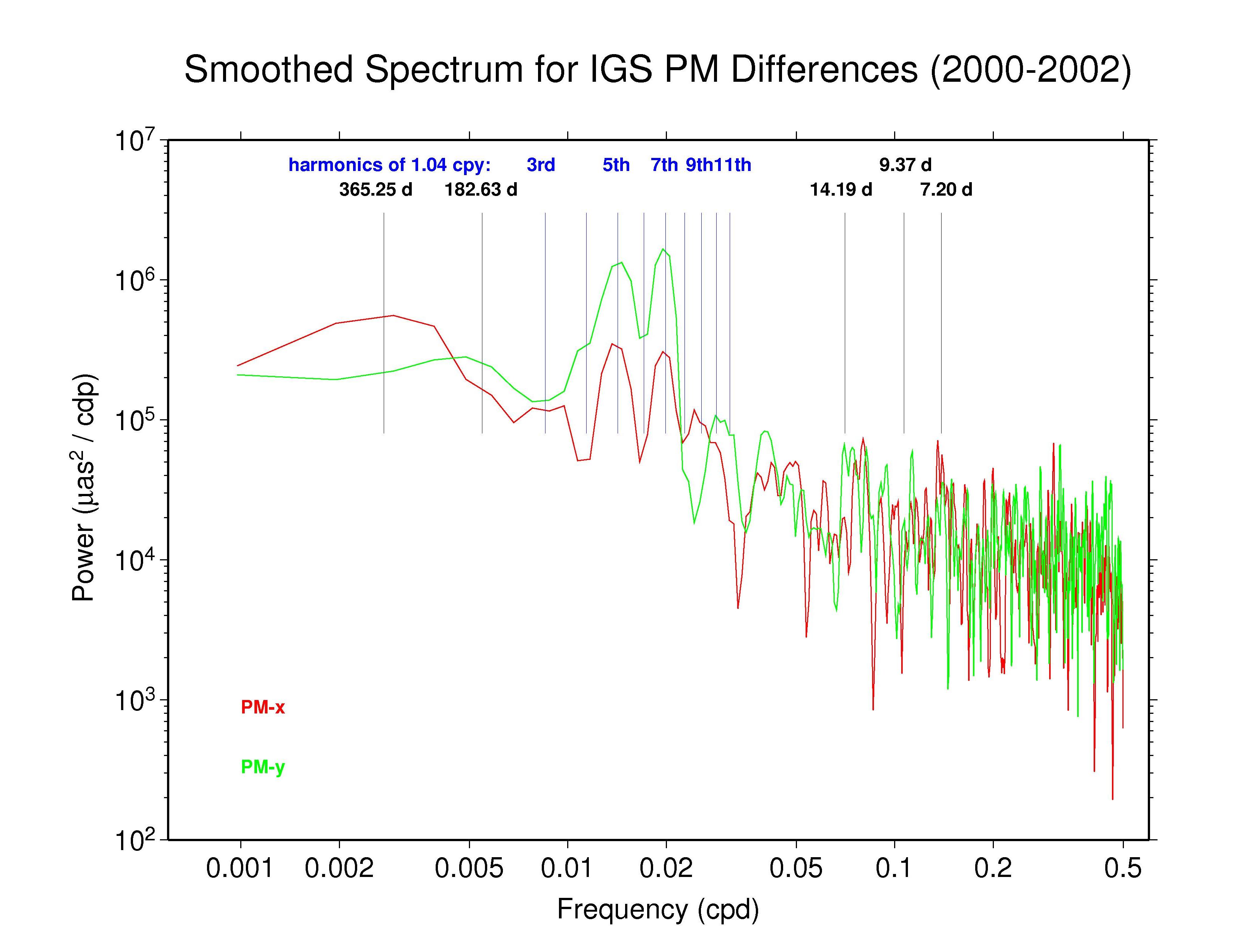
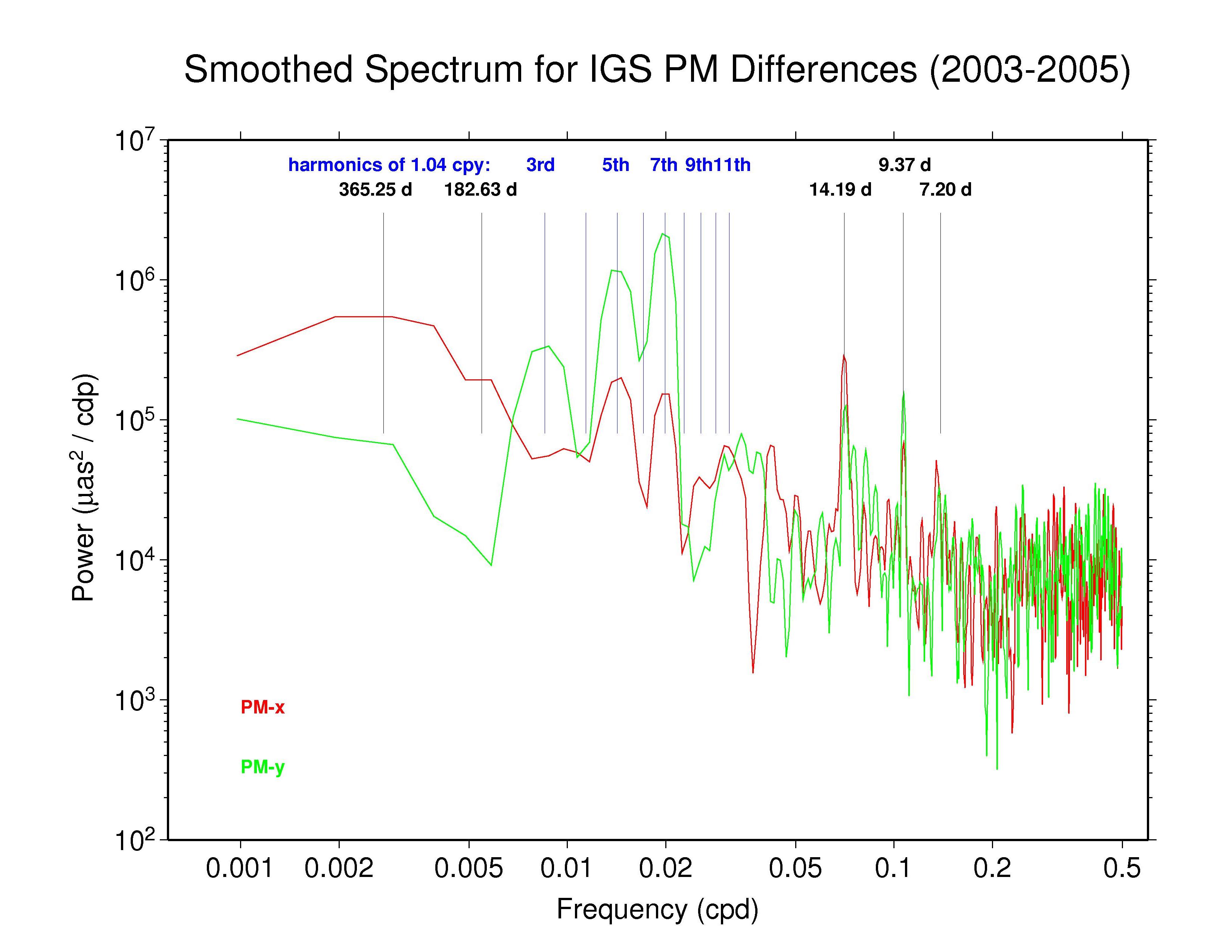
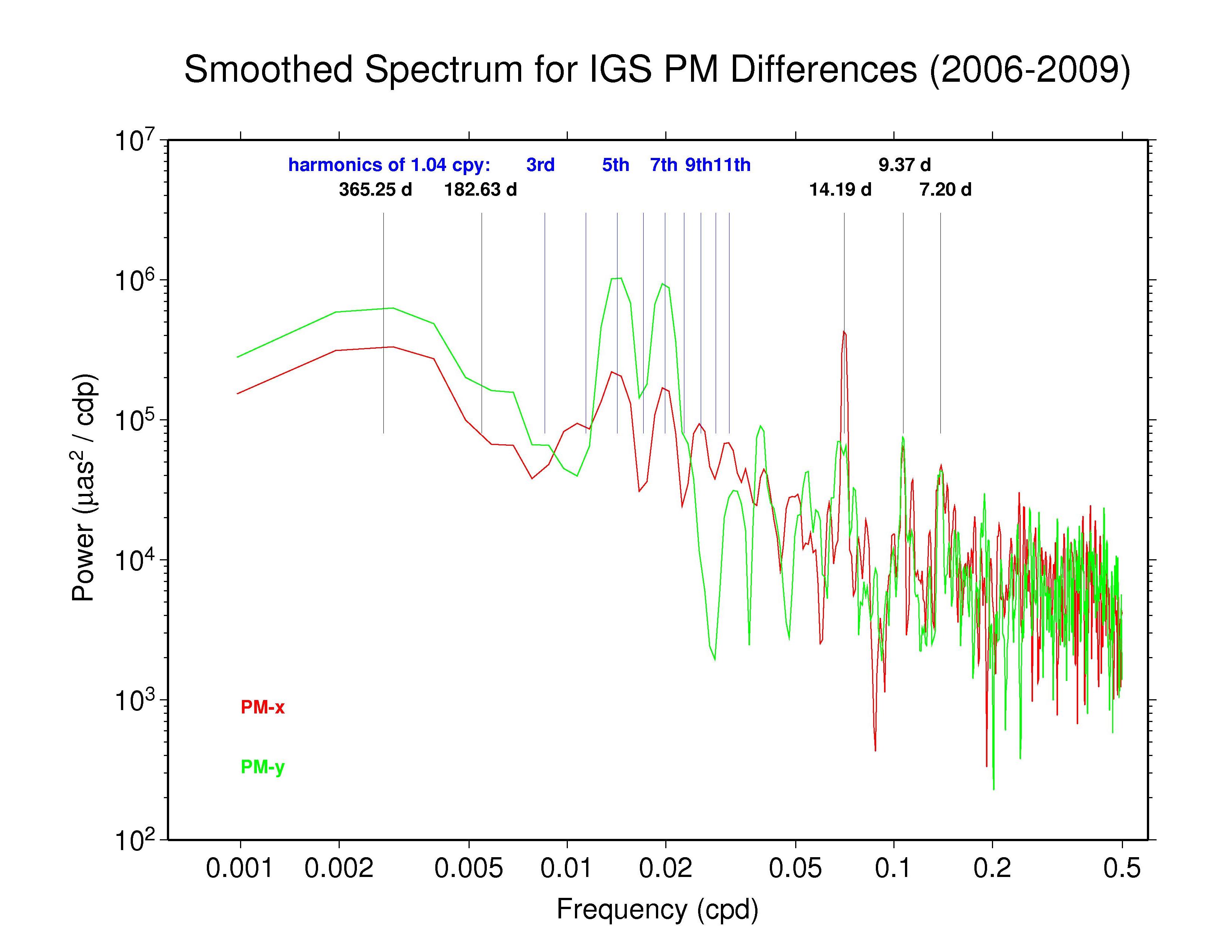
Spectra of IGS Polar Motion Discontinuities at Day Boundaries
Obvious from the discontinuity plots above is the fact that the distributions of polar motion differences at day boundaries display clear systematic variations and do not obey white noise statistics. This is an indication, among other things, of longer-term biases in the polar motion rate estimates, presumably reflecting deficiences in the data modeling, especially the orbit and a priori EOP modeling.
Spectra of the day-boundary differences in polar motion are plotted below, using red for the PM-x component and green for the PM-y component. In each case a boxcar filter has been used to smooth across each three adjacent frequencies. Some interesting spectral lines are also marked in each plot.
 IGS (1997-1999) —
ps file IGS (1997-1999) —
ps file
|
 IGS (2000-2002) —
ps file IGS (2000-2002) —
ps file
|
 IGS (2003-2005) —
ps file IGS (2003-2005) —
ps file
|
 IGS (2006-2009.5) —
ps file IGS (2006-2009.5) —
ps file
|
The table below summarizes the main features that can be observed in the spectra of the IGS polar motion discontinuity plots above. The ubiquity of the line near 14.2 d reminds us that Kouba (2003) showed that this can be an alias of any error in the adopted subdaily O1 tidal EOP model beating against the IGS 24-hr processing interval. Aliased subdaily tidal lines are considered in more detail in the earlier study by Ray (2009). In addition, Kouba (unpublished) previously showed that errors in the prograde fortnightly nutation model, at 13.66 d, which is among the largest modified terms in the IAU 2000 nutation model compared to the IAU 1980 model, will alias into a retrograde 13.66 polar motion rate error. The latter error is not readily apparent, though. Note that the resolution of the spectra above is about 0.2 d in the fortnightly band, so 14.2 and 13.66 d peaks should be distinguishable.
| Features in Spectra of IGS Day-boundary Polar Motion Discontinuities | ||||||
| Interval | component | annual | semi-annual | tidal alias lines | 1.040 cpy harmonics | |
| 1997-1999 | PM-x | Y | - | - | 5th, 7th | |
| PM-y | Y | - | - | 5th, 7th | ||
| 2000-2002 | PM-x | Y | - | ? | 3rd?, 5th, 7th | |
| PM-y | - | ? | ? | 5th, 7th | ||
| 2003-2005 | PM-x | Y | ? | 14.2, 9.4, 7.2? | 5th, 7th | |
| PM-y | - | - | 14.2, 9.4, 7.2? | 3rd, 5th, 7th | ||
| 2006-2009.5 | PM-x | Y | - | 14.2, 9.4, 7.2? | 5th, 7th | |
| PM-y | Y | - | 14.2?, 9.4, 7.2? | 5th, 7th | ||
In my previous examinations of reprocessed IGS polar motion results I have been inclined to accept the interpretation by Kouba (2003) that the narrow spectra features seen above are probably caused by aliasing of errors in the adopted subdaily EOP tide model. (For an elaborated list of the expected alias features, see the table of values provided Richard Ray, private communication March 2009, available at Ray (2009).)
That hypothesis still seems justified considering that the particular alias features predicted if the IERS2003 EOP tide model has significant errors are actually seen in the IGS spectra. For instance, the plots below show spectra differences when comparing the IERS2003 EOP tide model with test models kindly provided by Richard Ray (private communication, 2009) using tide heights from the TPXO7.1 and the GOT4.7 global tide models. (Full hydrodynamic model reconstructions of ocean currents were not updated for these tests.) By synthesizing pseudo-observations of subdaily polar motion variations using the old and new tide models at 5-minute intervals, the expected impact on GPS estimates of polar motion and polar motion rates were computed and the model-only day-boundary discontinuities found. Their spectra are shown below. This simplified treatment assumes that no part of the subdaily EOP tidal effects are absorbed into any other parameters, which is certainly not valid at the K1 and K2 (near the GPS orbital) periods. But the latter have alias lines at annual and semi-annual periods, respectively, not in the sub-monthly band of prime interest here.
In this view, the narrow 14.2 d, 9.4 d, and 7.2 d spectral features for recent IGS results could be evidence for significant errors in the IERS2003 subdaily EOP tidal model for, respectively: O1; Q1 and/or N2; and σ1, 2Q1, 2N2, and/or μ2. In addition, at least some part of the large, broad annual power in the IGS discontinuities could be caused by errors in the EOP tides at K1 especially and perhaps P1 and T2.
One aspect of the new observations that is difficult to understand as a purely alias effect is the apparent growth of the 14/9/7 d lines in more recent data. The EOP tides should be stationary for very long periods and their alias features would not be expected to grow in amplitude, as they clearly do. The higher background noise of the earlier estimates could obscure the presence of alias features somewhat, but this cannot be a complete explanation based on a comparison of the relevant amplitudes. The fortnightly line during 2006-2009 should definitely be visible during 2000-2002 and perhaps earlier. Instead, the new results presented here may require the presence of an effect in addition to subdaily tidal aliasing.
Part of the apparent time variability could be due to an evolving relative mix of AC solutions used in the IGS combinations, each with different sensitivities to the tidal errors. This would only seem plausible if some ACs have applied sufficiently strong continuity constraints that the tidal alias errors were effectively dampened and if those contributions have received heavier relative weights in the older periods. However, this condition seems opposed to the observation of stronger combined smoothing near the Nyquist frequency in the more recent data, rather than in the older.
In view of the weekly modulation of the IGS polar motion and polar motion rate formal errors, discussed above, which points to effects in the AC analysis procedures, it is tempting to consider if 7 and 14 d artifacts might contribute to the day-boundary discontinuity spectra. The available spectral resolution is not adequate to rule out a mix of artifactual and aliased signals, with the artifactual component having grown in more recent years. For the moment, a hybrid theory is my preferred explanation: subdaily EOP tide model aliasing errors are present (as clearly evidenced by the 9.4 d peak in recent data), but their expression changes over time due to the varying weights of different AC contributions, some of which have dampened the subdaily alias errors by continuity constraints while others possess artifactual signals from the 7 d weekly processing cadence.
The much broader bands seen in the day-boundary discontinuities with periods between about monthly and semi-annually, especially for PM-y, correspond mostly to the 5th and 7th harmonics of the GPS draconitic, 1.040 cpy (or 351 d period). Therefore, it is probable that these features near 70 and 50 d periods, respectively, are related to orbit mismodeling errors. It is not clear why the 5th and 7th multiples, in particular, are stimulated above any others, nor why the PM-y component is much more strongly affected than PM-x.
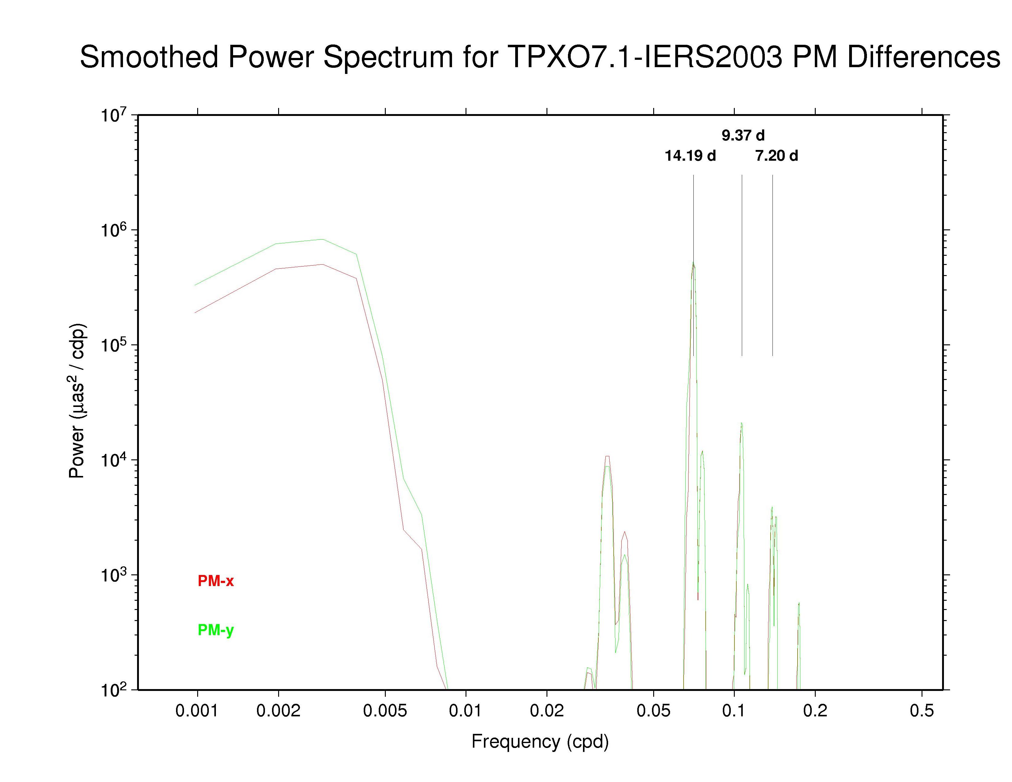 TPXO7.1 - IERS2003 EOP tide model differences —
ps file TPXO7.1 - IERS2003 EOP tide model differences —
ps file
|
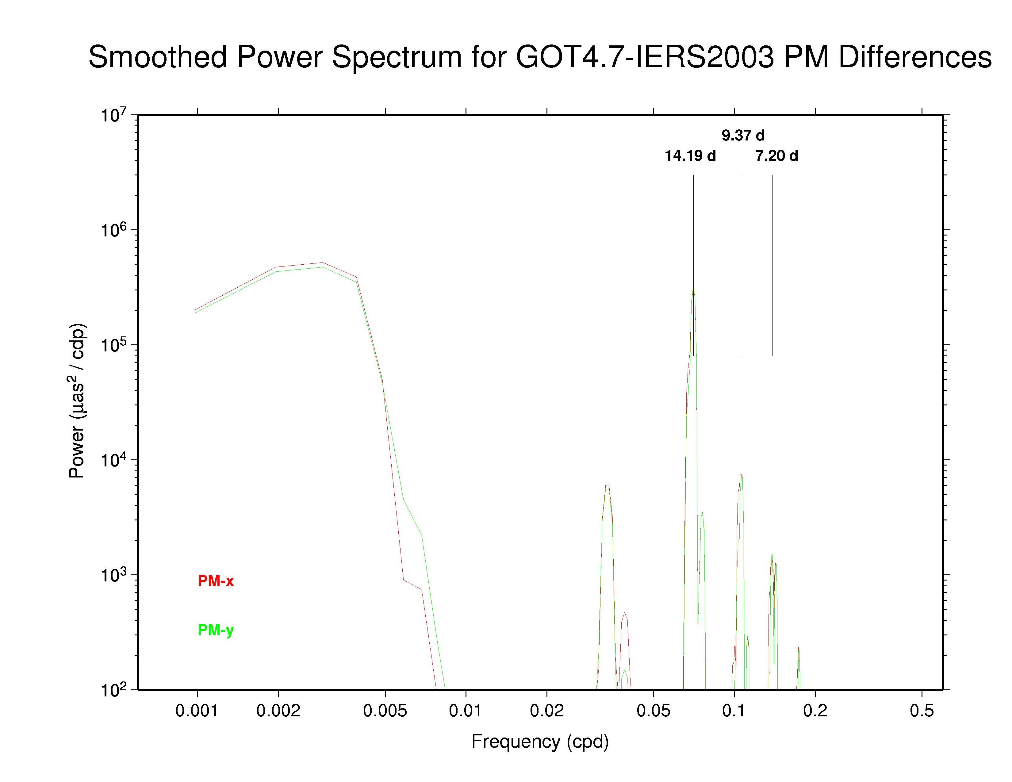 GOT4.7 - IERS2003 EOP tide model differences —
ps file GOT4.7 - IERS2003 EOP tide model differences —
ps file
|
| Send comments to Jim Ray | (updated 25 August 2009) |