 |
|
|
| |
|
|
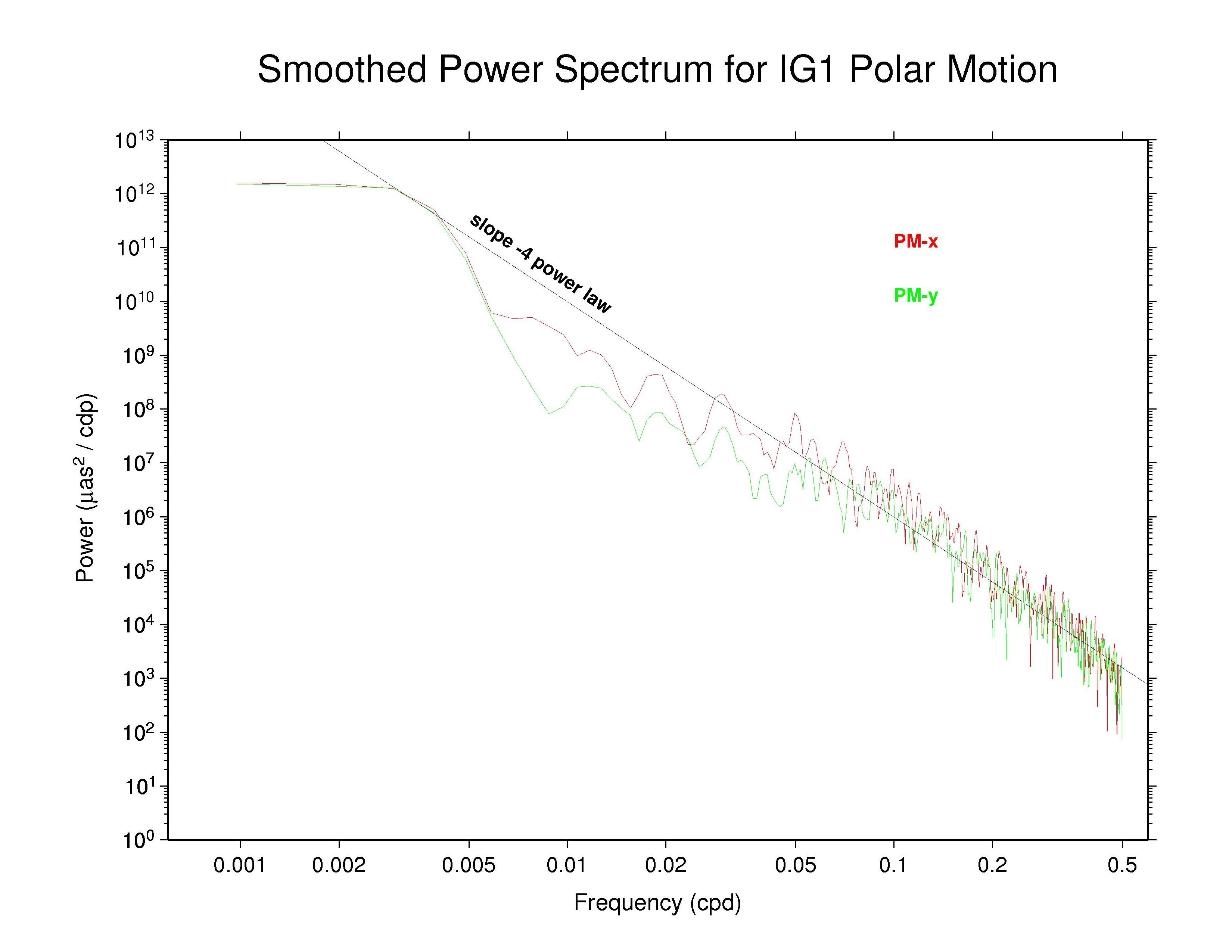
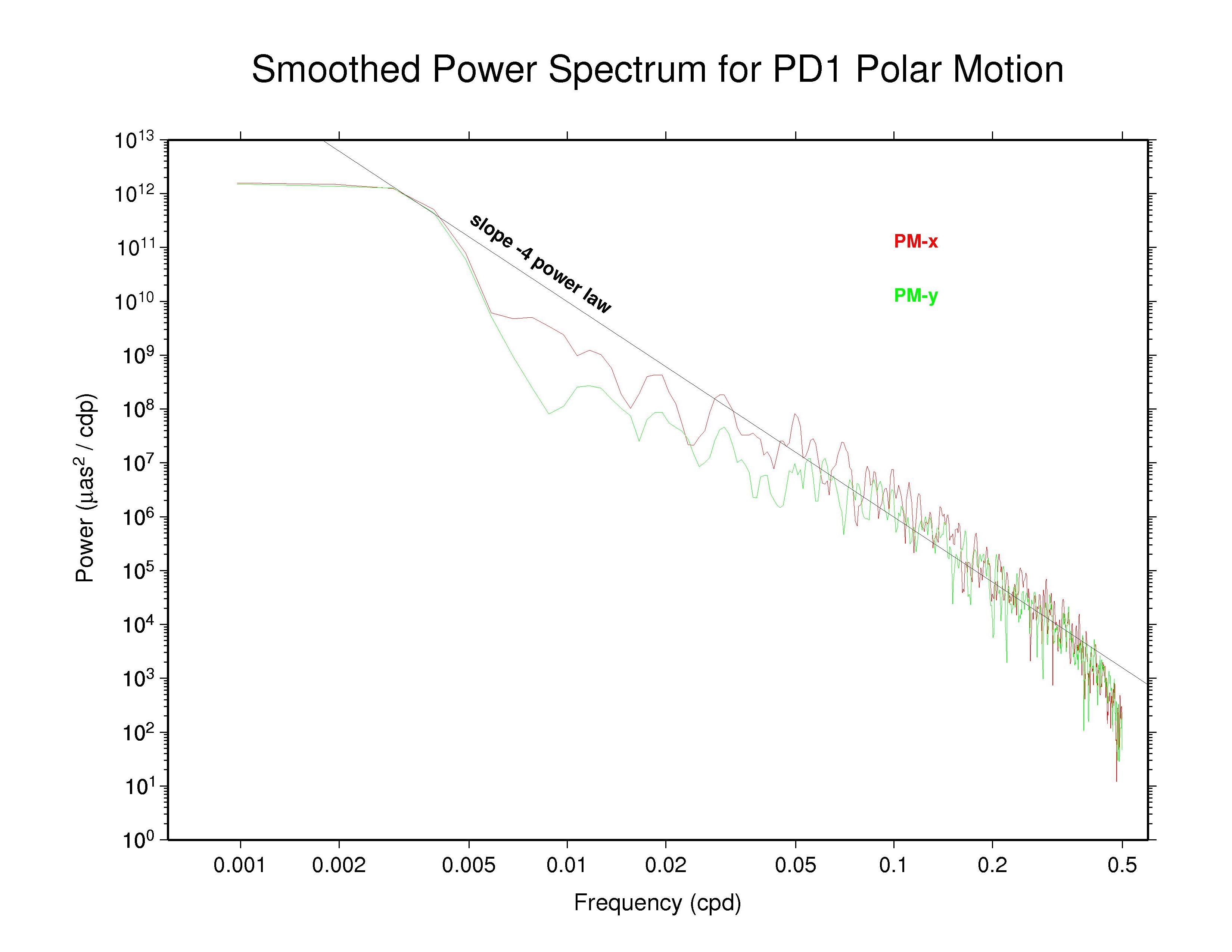
Power spectra have been generated and are plotted below for the polar motion time series of each Analysis Center (AC) participating in the IGS Reprocessing Campaign #1 (repro1), as well as for the IGS combination. A matching site to this one looks at the associated orbit discontinuity time series. The 1024 days (or 1025 days for differences) through week 1459 (end of 2007) have been used to obtain consistent, comparable, and modern results from all ACs. This span covers epochs from MJD 53440.5 (or 53439.5 for polar motion differences) through 54463.5, which corresponds to the period 11 (or 10) Mar 2005 (week 1313_5) through 29 Dec 2007 (week 1459_6). Polar motion values have been extracted from the reported weekly ERP files and assume that the ERP estimates are freely estimated without any constraints. In the case when the associated SINEX ERP values are actually reported with non-trivial constraints, the effect of those constraints (which are removed in the official SINEX combination) is not accounted for here. This consideration applies in particular to the PDR ERP values (see more below). Note that for those ACs reporting 9 ERP values each week, the 7 unique middle values have been used here.
The results presented here can be compared with a previous study of IGS operational polar motion results by Ray (2008), which covered nearly the same time period: the 1024 days from MJD 53412.5 (week 1309_5 or 11 Feb 2005) to 54435.5 (week 1455_6 or 01 Dec 2007). The consequences of polar motion smoothing by imposition of day-to-day continuity constraints was discussed in considerable detail there.
For these displays a smoothing across each three adjacent frequencies has
been applied with a sliding boxcar filter to make the appearance less noisy
(but unsmoothed plots are also available and are not substantially
different). In each case, the smoothed
spectrum for the x component of polar motion is shown as the red curve and
the y component is shown in green.
Most continuous geophysical processes and most physical noise processes
possess power spectra that decrease as the frequency raised to some
characteristic negative power ("spectral index"). The spectra are usually
"reddish" in the sense of having more power at the lower frequencies
(i.e., longer periods). For reference, a power law with spectral index
of -4 is drawn on each plot (not a fit). This corresponds to the
behavior of an integrated random walk (in phase) noise process, that is,
a doubly integrated white noise process.
  IGS —
ps file IGS —
ps file
|
 CODE —
ps file CODE —
ps file
|
 EMR —
ps file EMR —
ps file
|
 ESA —
ps file ESA —
ps file
|
 GFZ —
ps file GFZ —
ps file
|
 GTZ —
ps file GTZ —
ps file
|
 JPL —
ps file JPL —
ps file
|
 MIT —
ps file MIT —
ps file
|
 NGS —
ps file NGS —
ps file
|
 PDR —
ps file PDR —
ps file
|
 SIO —
ps file SIO —
ps file
|
 ULR —
ps file ULR —
ps file
|
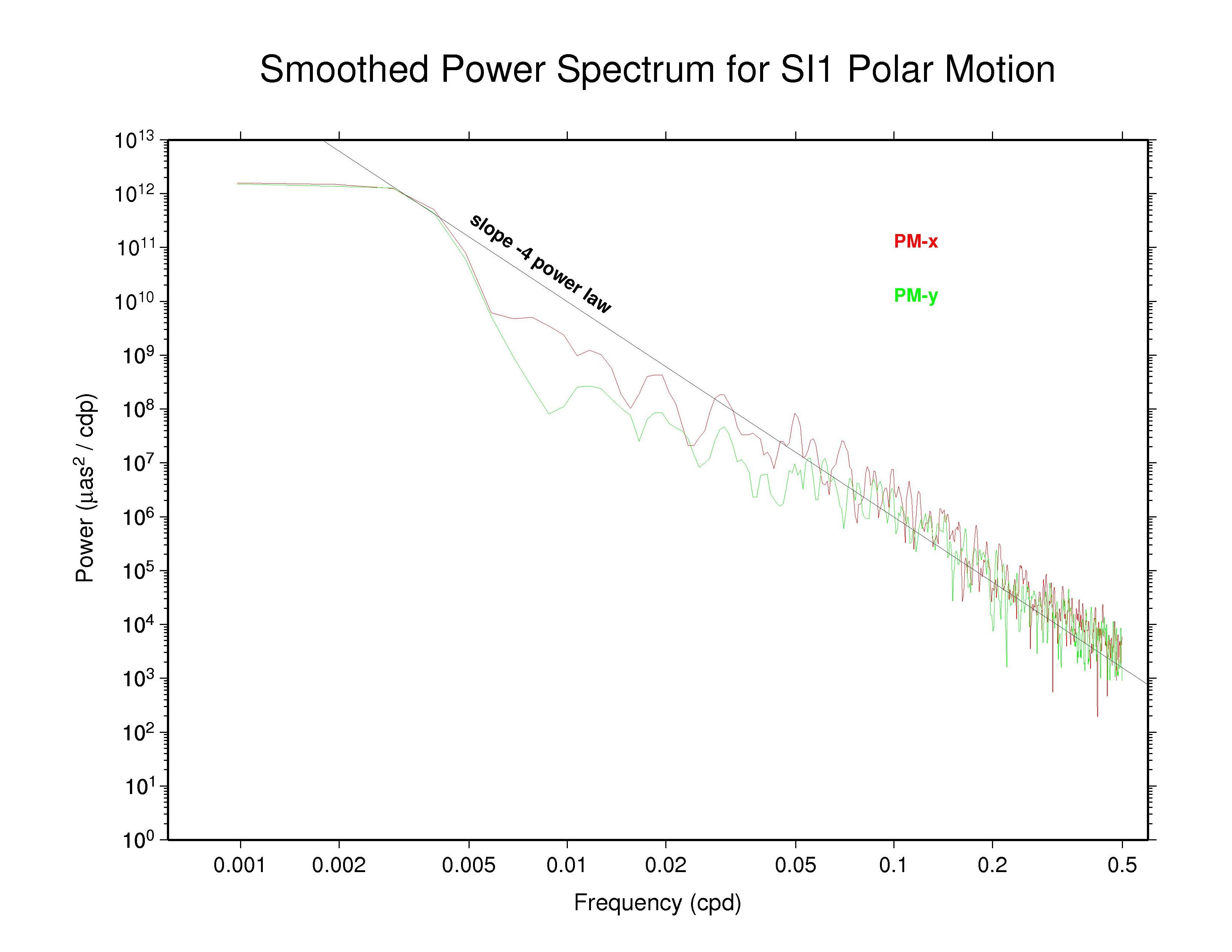
Of these AC polar motion spectra, most show completely nominal
characteristics; that is, their spectra follow a single power-law for
periods shorter than about 20 days with spectral index close to -4.
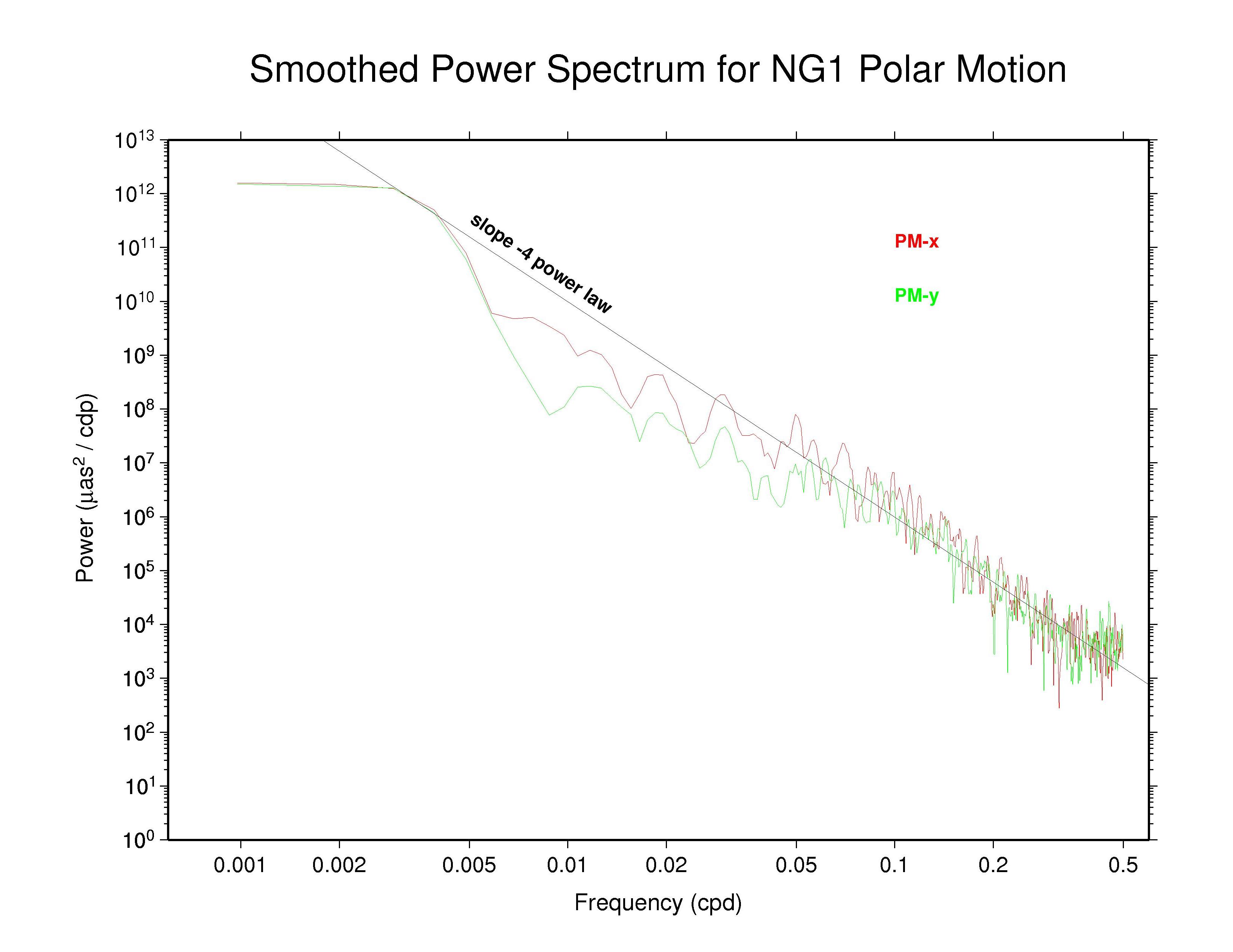
Some ACs (particularly NGS) show nearly power-law behavior over most
of the high-frequency range but also display some slight spectral
flattening as frequencies approach the Nyquist limit of 0.5 cpd,
presumably the effect of a modest white noise floor.
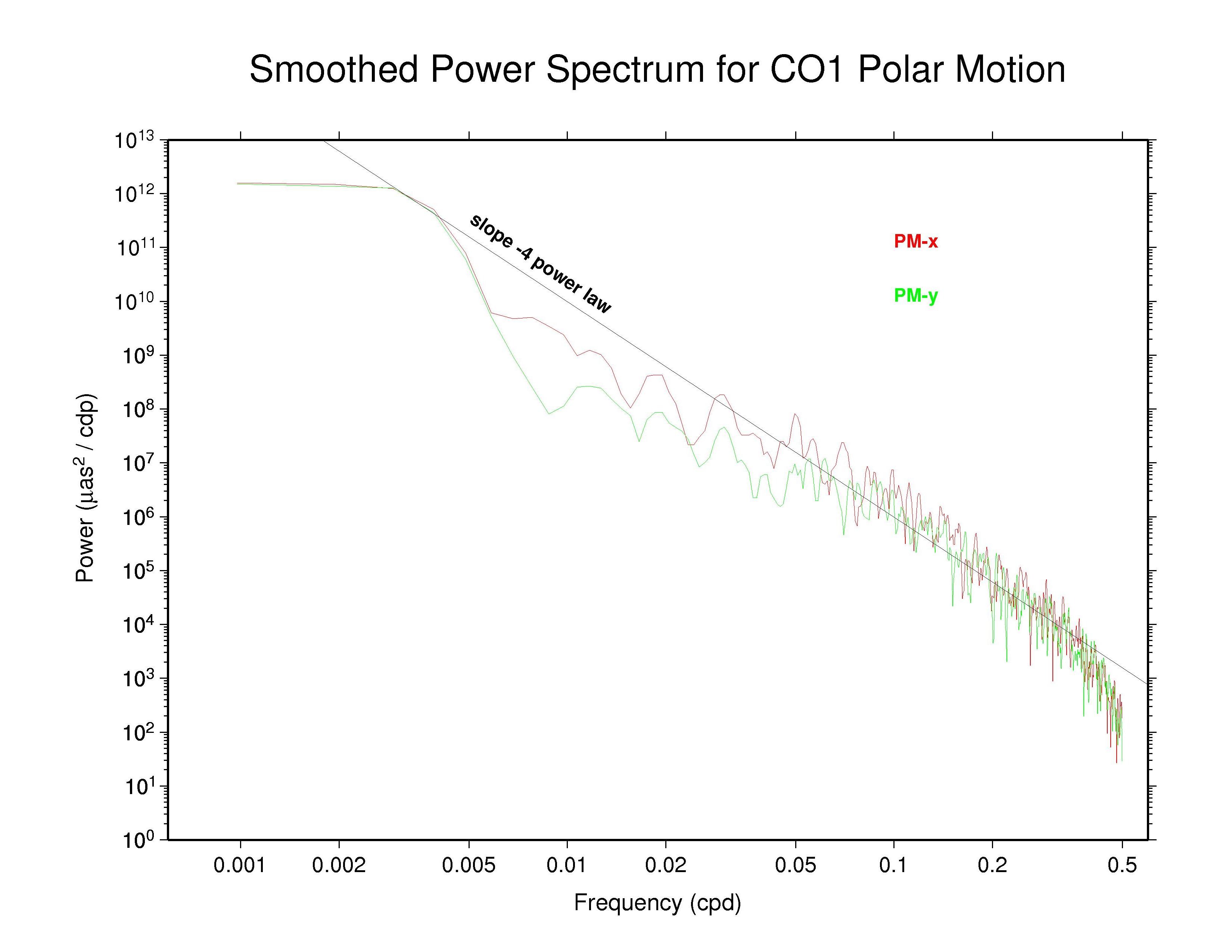
The gradual but sharp steepening of the CODE and PDR power spectra at the
highest frequencies illustrates the high-frequency smoothing/filtering
effect caused by imposing a strict day-to-day continuity condition on
the estimates of the polar motion rate parameters. This is true for the
values reported in the PDR ERP files, which were also used in the weekly
PDR back-solutions to generate consistent products for satellite orbits,
clocks, etc (Mathias Fritsche and Peter Steigenberger, private
communication February 2009). However, the official PDR ERP values are
those reported in their SINEX files together with station coordinates and
full variance-covariance information. Those SINEX ERP values are reported
with tight (but removable) constraints of about 13.5 µas and 13.5
µas/d. In this way the PDR ERP continuity constraints do not
actually disturb the IGS ERP combination, and the plots shown here do not
properly represent the actual PDR polar motion behavior after removal of
the constraints. On the other hand, the continuity conditions applied
in the CODE analysis are not removable and using these results in the IGS
combination would smoothen the official values. The consequences have
already been considered in a previous study of IGS operational polar
motion results (Ray, 2008). For that reason,
the CODE ERP estimates are excluded from the IGS combination.
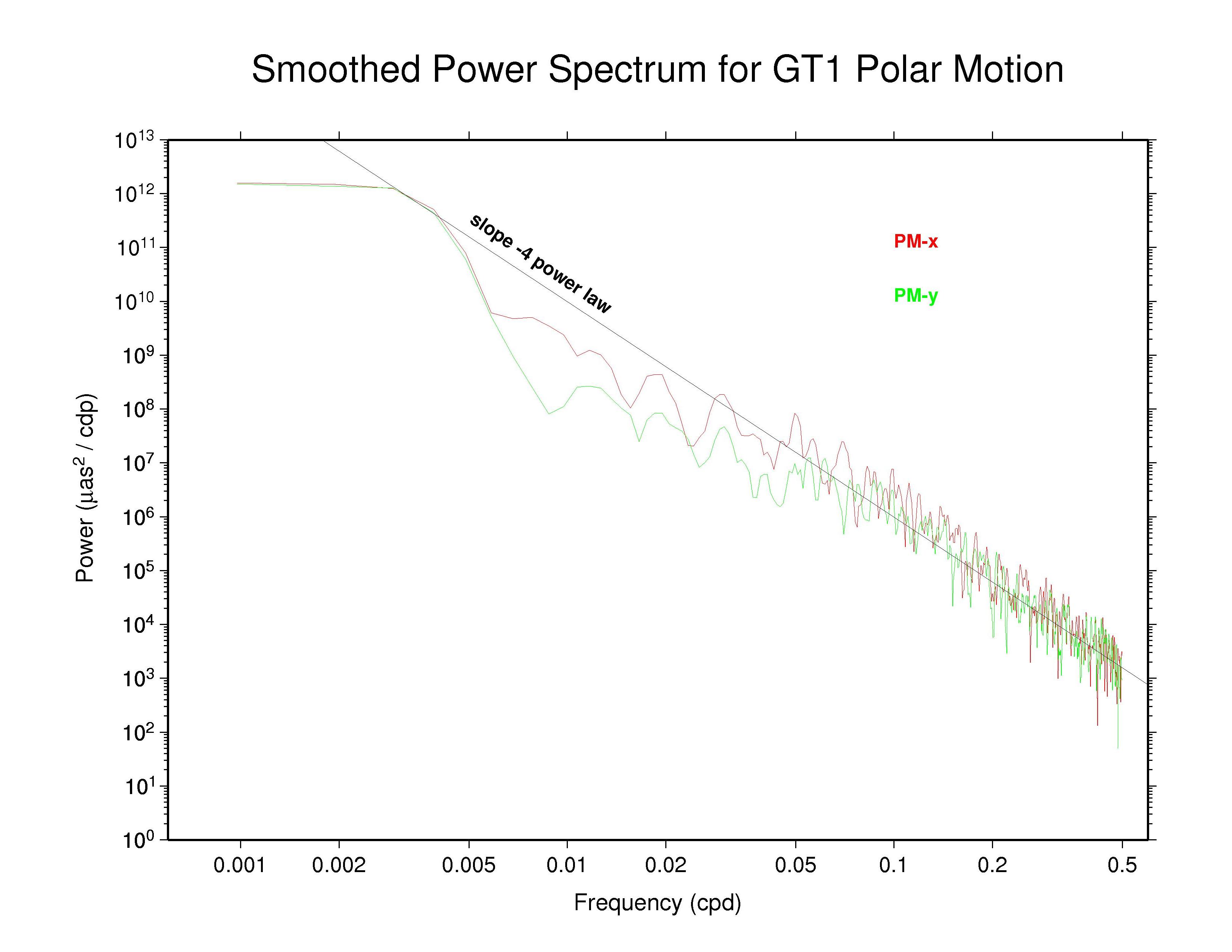
It is possible that the GFZ and maybe the GTZ spectra show very slight indications of some high-frequency smoothing also, but that is uncertain from the power distributions alone.
Day-boundary Discontinuities in Polar Motion Series
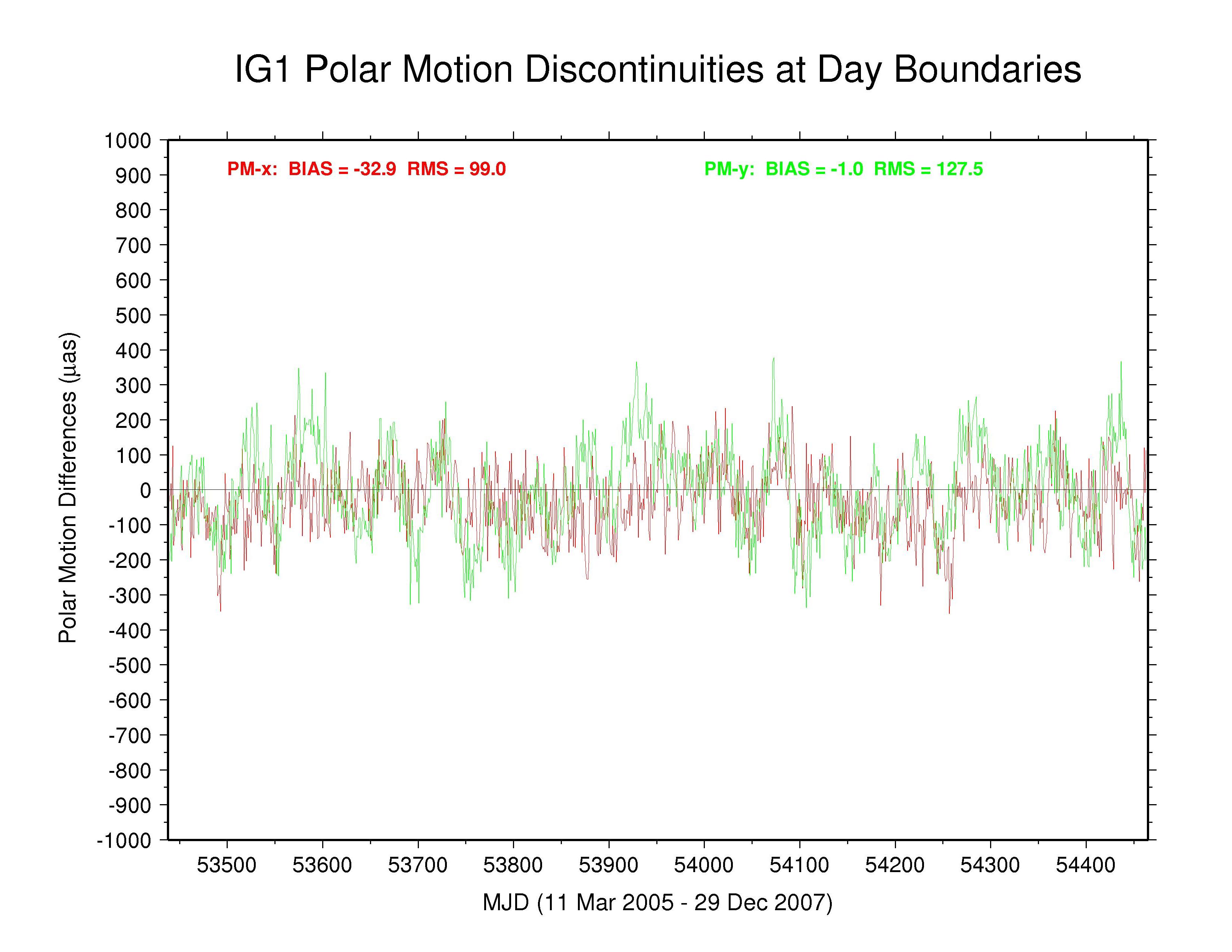
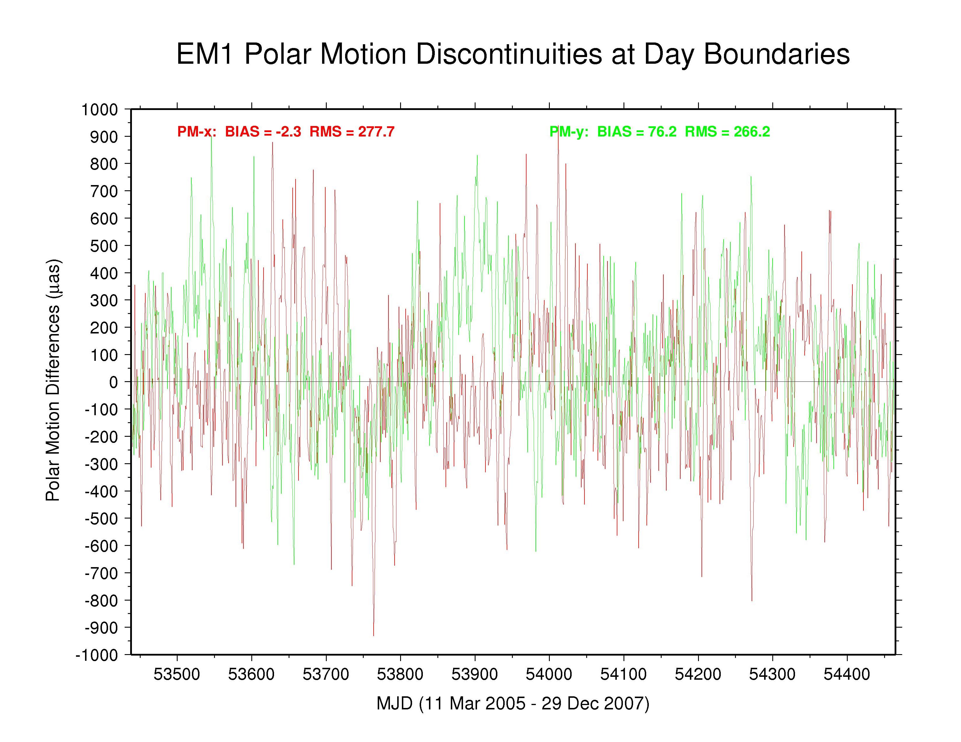
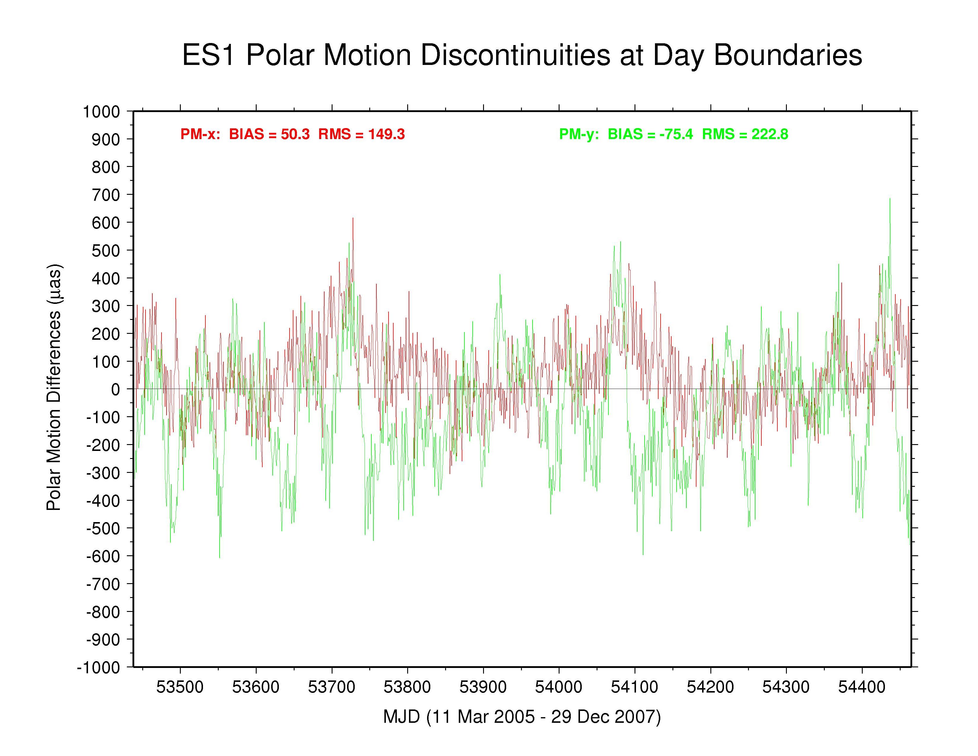
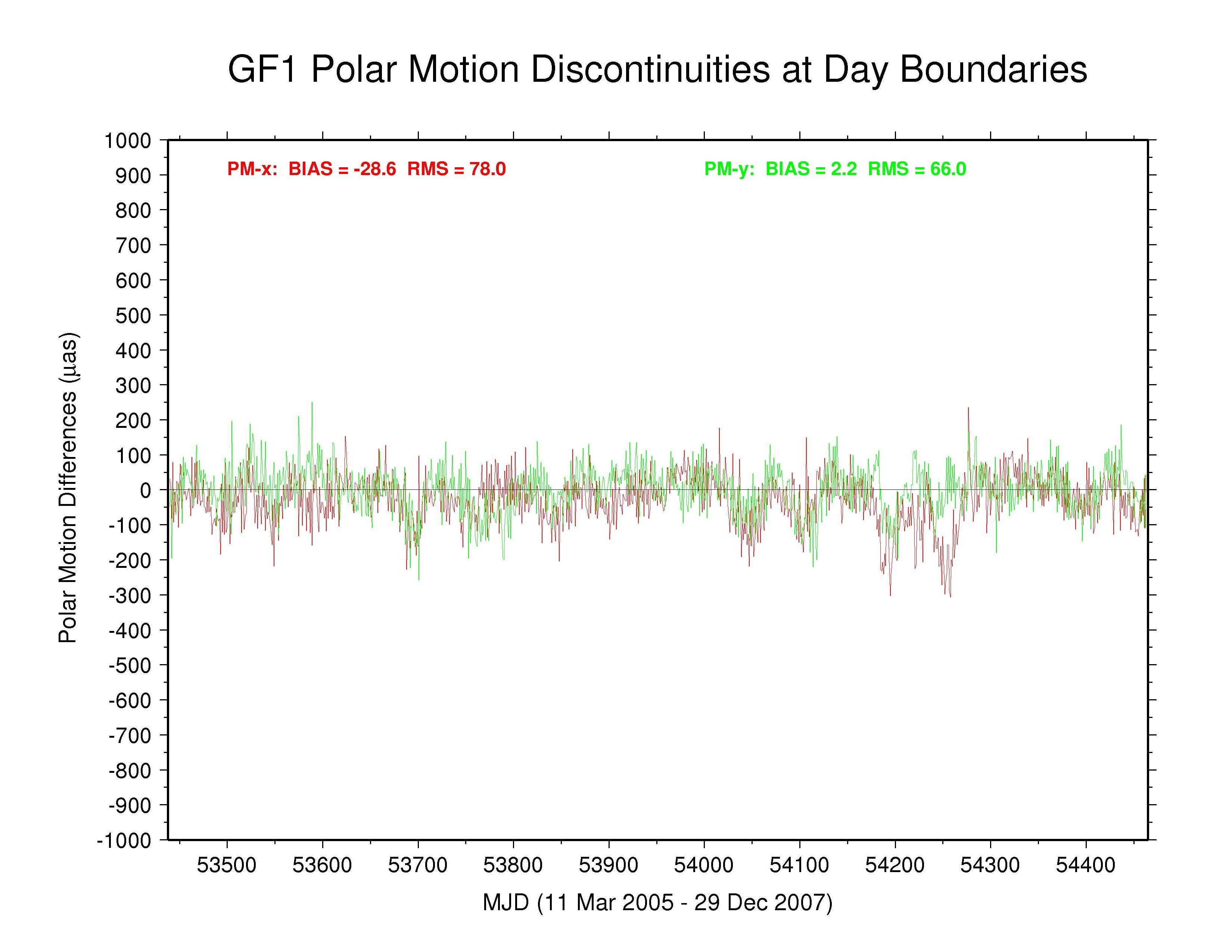
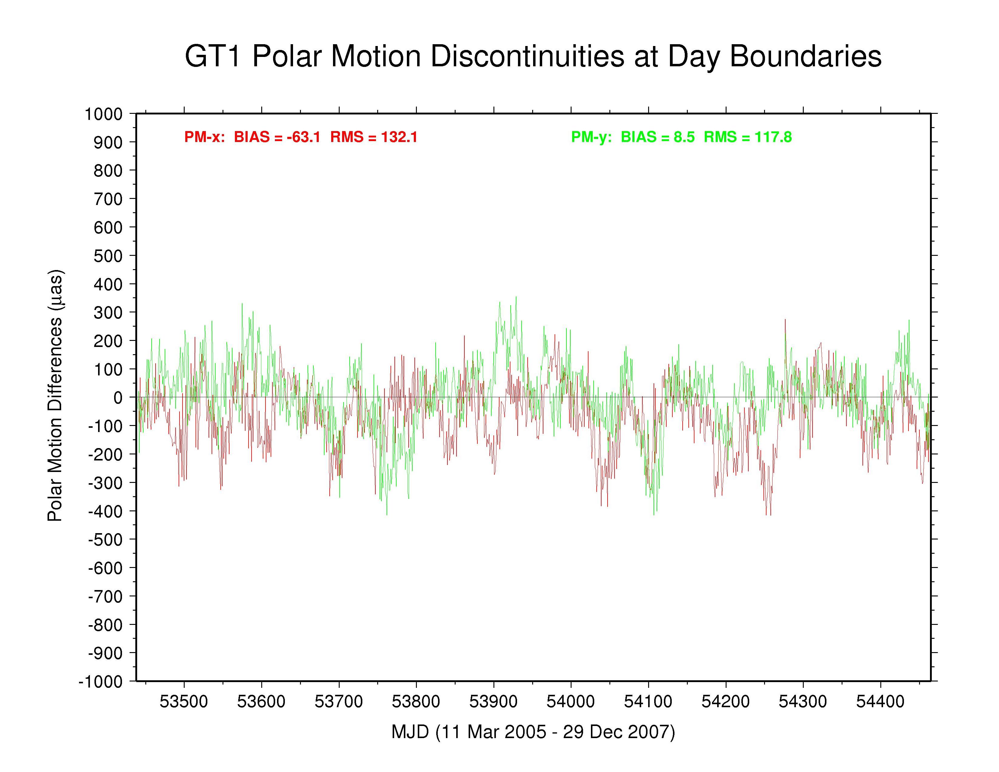
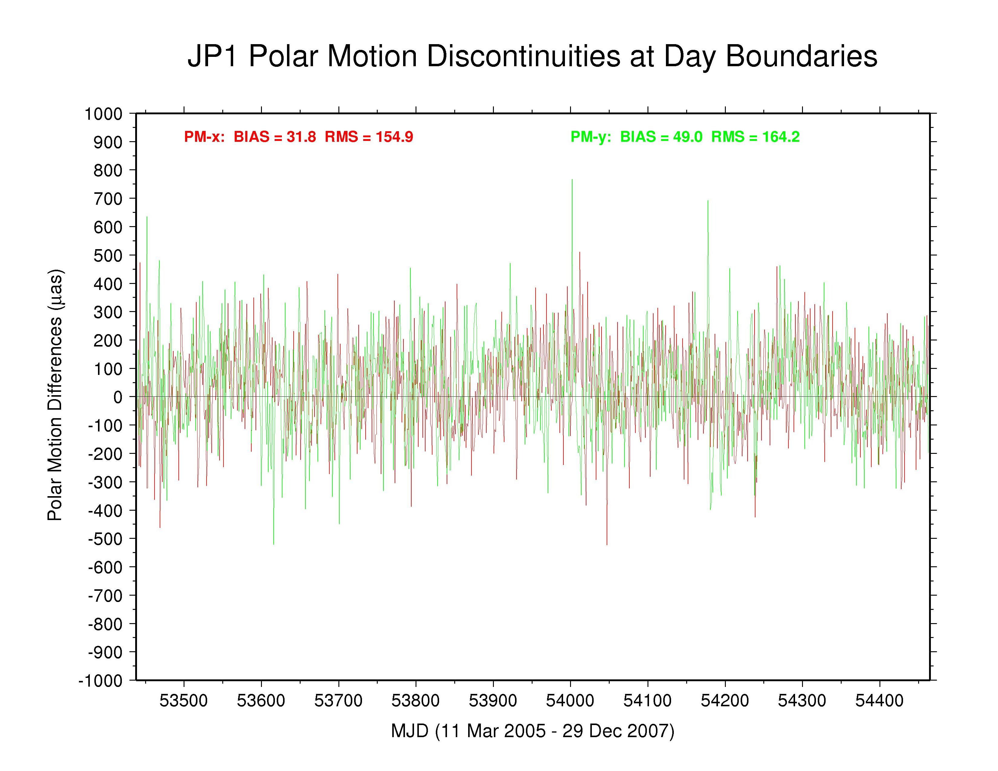
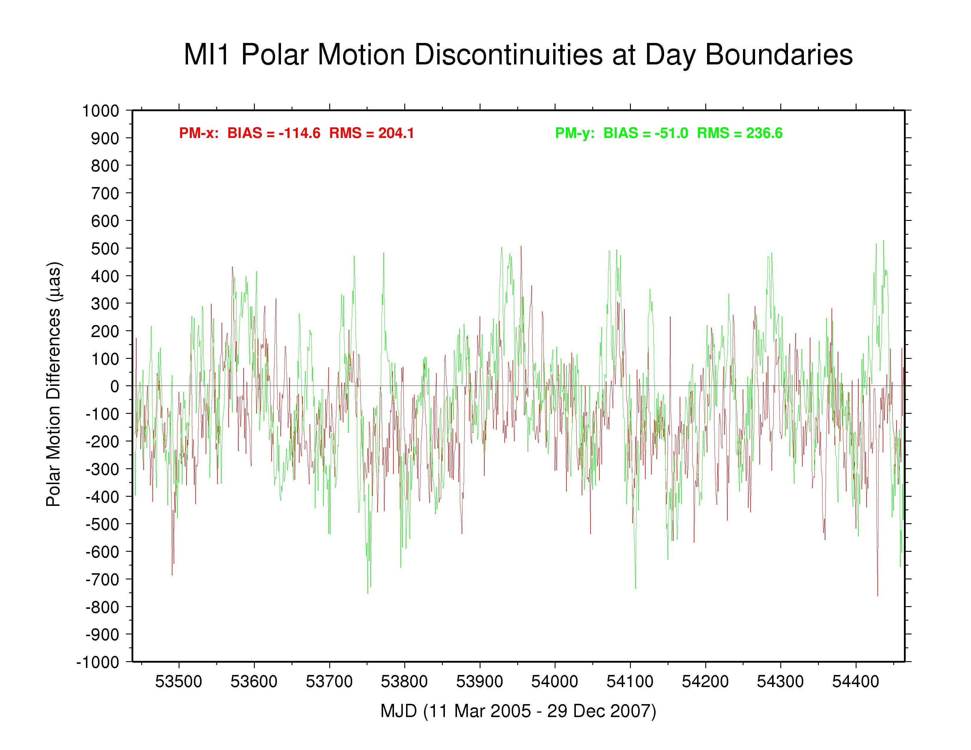
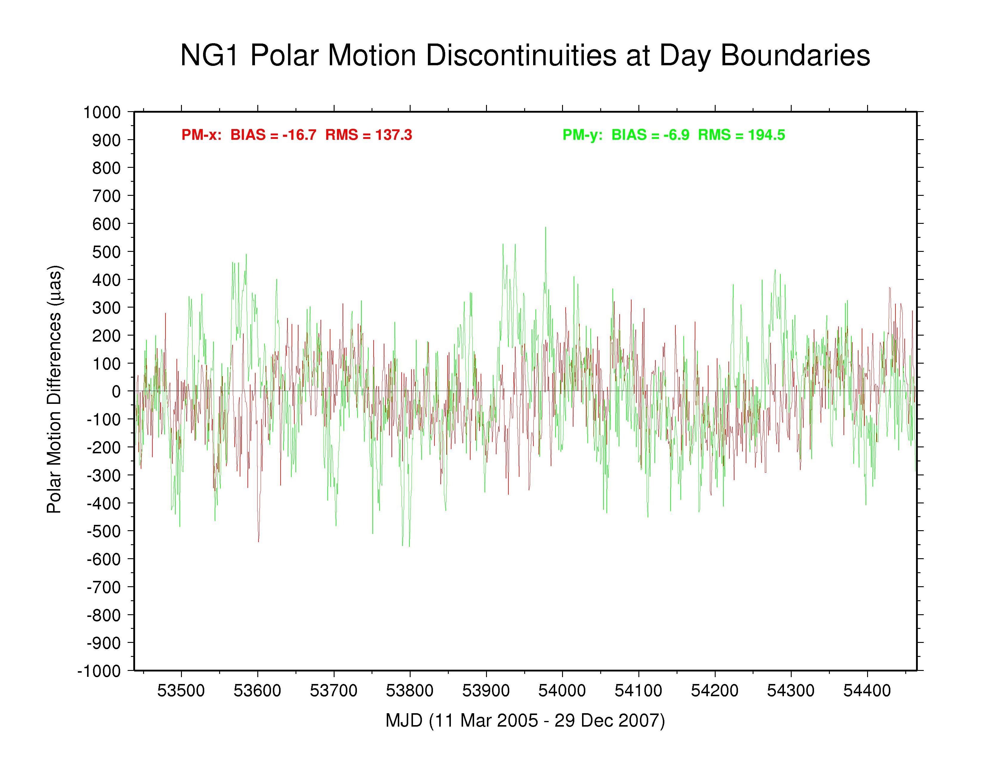
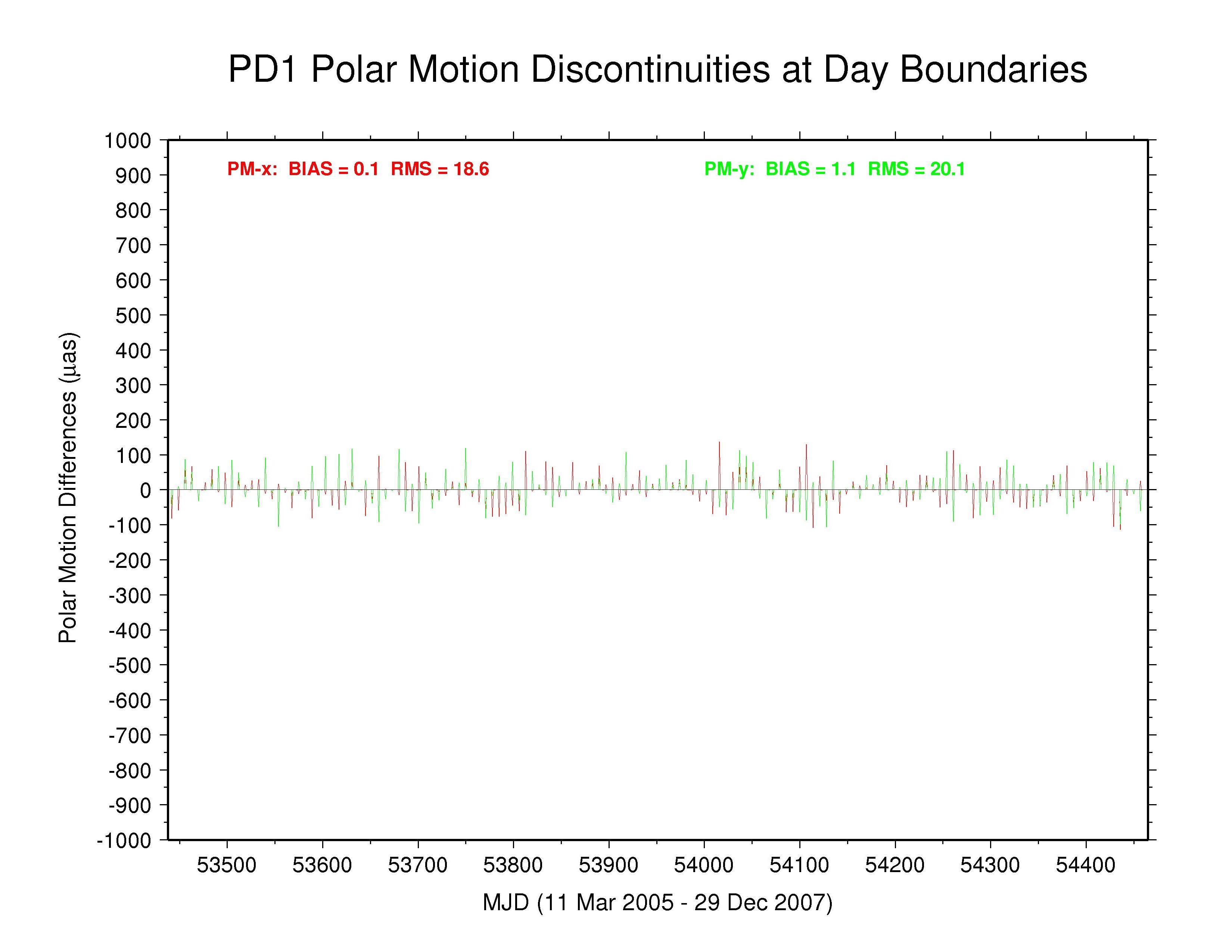
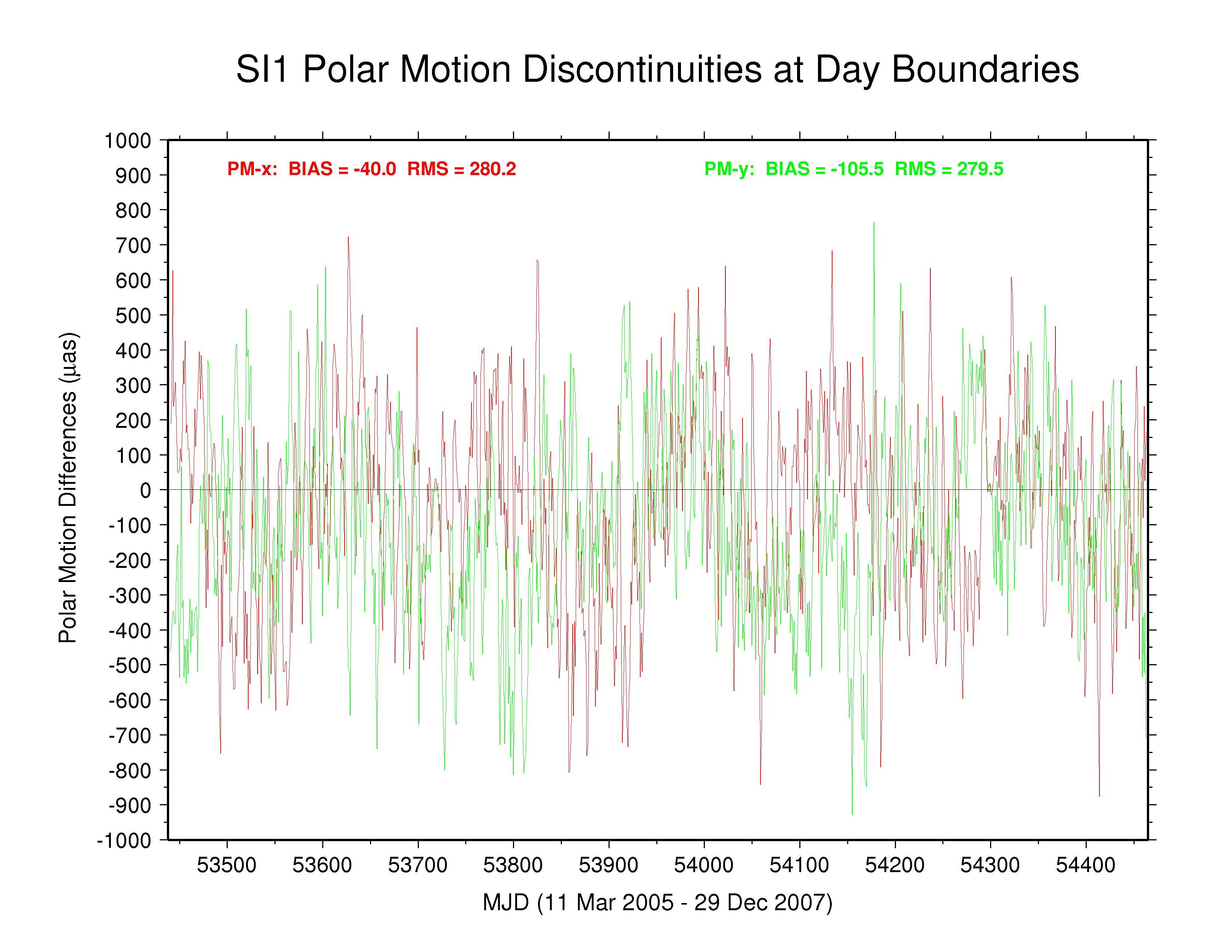
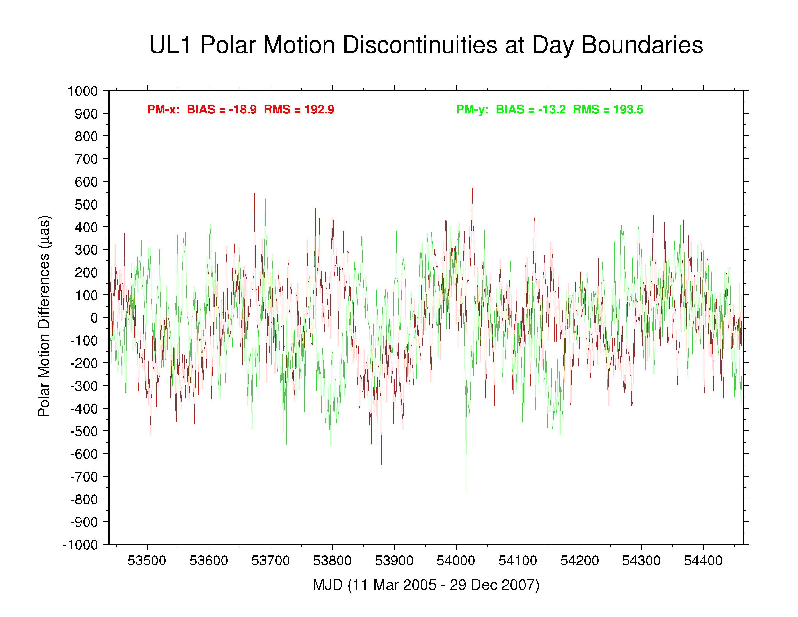
To examine the extent to which continuity conditions have been imposed on the polar motion rate parameters between days (and for other reasons), the discontinuities in the polar motion time series have been computed at day boundaries and plotted below. The differences at each midnight epoch were found by [PM(day2) - (0.5*PMrate(day2))] - [PM(day1) + (0.5*PMrate(day1))] for each successive pair of days, day1 and day2. x component discontinuities are shown in red while y component discontinuities are shown in green. On each plot is also shown the (unweighted) mean bias and RMS for each component and each AC, as well as for the IGS combination. It should be noted that the polar motion offset and rate values used here are those from the respective ERP files. If any removable ERP constraints have been reported in the AC SINEX files, which are the source of official estimates, those have not been accounted for here. However, the constraint values in SINEX files with reported ERP constraints are very loose and should not affect these results (except for PDR as explained above).
Note that the dispersion in AC performances shown here reflects almost entirely the behavior of their polar motion rate estimates, not the mid-day polar motion offsets. As long as no strong continuity constraint is imposed on the rate estimates, their variations (for whatever reason) probably have minimal impact on the associated mid-day (also mid-arc) polar motion offset estimates. This means that end-users of IGS polar motion results should probably rely more heavily on the offset values and not on the rate values, even for studies of geophysical excitation (that is, polar motion rate-of-change). It is probably more reliable to use polar motion change estimates derived from fits to the offsets (via splines, for instance) than to use the directly estimated polar motion rates for reasons that will be demonstrated in the next section.
Polar motion rate estimates are probably most useful as a probe of the quality of the AC modeling, especially the modeling of the satellite orbit dynamics, and the a priori subdaily EOP model reliability than as accurate measures of Earth dynamics. Since a pole position offset is sensed in the GNSS modeling as a global diurnal sinusoidal motion of the terrestrial frame relative to the satellite frame, any similar type constellation-wide errors in the orbital frame can alias into the polar motion and polar motion rate estimates. Satellite methods are completely incapable of detecting diurnal retrograde motions, which for the Earth correspond to nutations. Consequently, it is also useful to examine the spectra of the polar motion discontinuities to see if these reveal information about data modeling deficiencies (see next section).
 IGS —
ps file IGS —
ps file
|
 CODE —
ps file CODE —
ps file
|
 EMR —
ps file EMR —
ps file
|
 ESA —
ps file ESA —
ps file
|
 GFZ —
ps file GFZ —
ps file
|
 GTZ —
ps file GTZ —
ps file
|
 JPL —
ps file JPL —
ps file
|
 MIT —
ps file MIT —
ps file
|
 NGS —
ps file NGS —
ps file
|
 PDR —
ps file PDR —
ps file
|
 SIO —
ps file SIO —
ps file
|
 ULR —
ps file ULR —
ps file
|
The behaviors of the polar motion discontinuities differ greatly among the ACs and the IGS combination. Mean bias and RMS values (unweighted) are tabulated below for each polar motion discontinuity time series. All the results show clear systematic patterns in the time variations of their polar motion discontinuities. Those of GFZ have the smallest overall scatter (except for the special cases of COD with strict continuity constraints and PDR where the continuity constraints have not been removed), even smaller than the IGS combination. Some moderate level of (weighted) continuity constraint is imposed in the GFZ estimation (Gerd Gendt, email 03 Jan 2008), which might explain their smaller level of variation. However, the a priori constraints reported in the GFZ SINEX files are only at the level of 103 to 104 mas or mas/d, which should have no noticeable impact. Considering that the RMS values for the GFZ PM discontinuities are considerably smaller than for the IGS combination, it appears that the effective GFZ continuity constraints must actually be much tighter than those reported, possibly due to some implicit constraints.
The situation with the GTZ discontinuities is similar to the other ACs for PM-x but more like GFZ for PM-y in having a smaller RMS than the IGS combination.
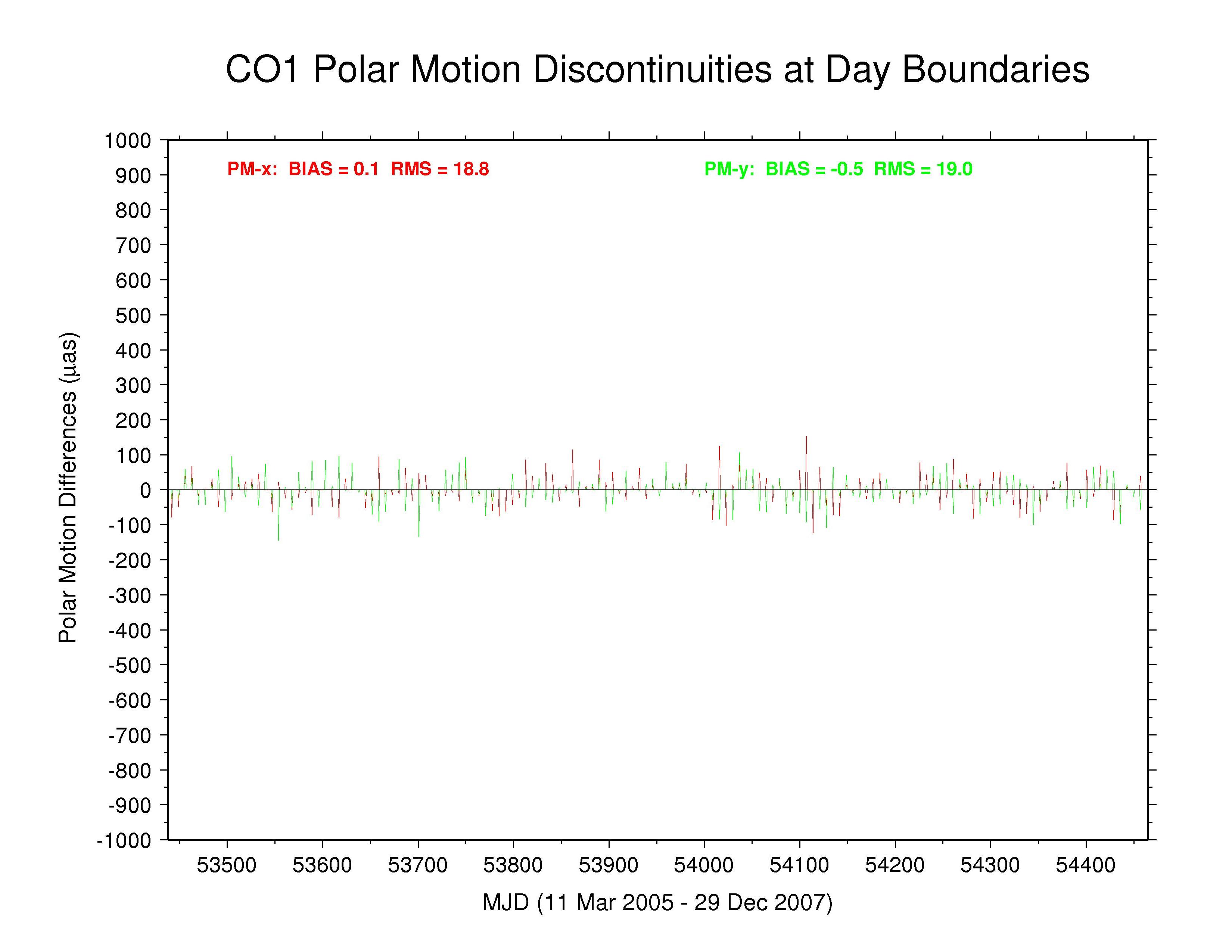
The effective smoothing in the COD and PDR polar motion spectra seen previously is caused by forcing strict continuity between adjacent days in the estimation of daily polar motion offsets and rates. This continuity condition has not been removed in the PRD results shown here and cannot be removed from the COD results. The discontinuities are not identically zero every day because both COD and PDR they report 9 values for each week and only the central 7 values have been used here. This causes the spikes seen once each week.
Significant long-term polar motion rate biases are seen below in several AC solutions. These are most noticeable for MIT in PM-x, with GTZ, ESA, and SIO being less so, and for SIO in PM-y, with EMR, ESA, and MIT being less so. Biases are smaller in both components for JPL and are relatively benign for GFZ and for GTZ in PM-y (though probably due in part to continuity conditions) and for NGS and ULR. From the smallest unquestionably unconstrained AC RMS values (about 150 µas for PM-x and about 200 µas for PM-y) we can infer the approximate internal accuracy of the AC polar motion rate estimates. We assume that the discontinuity scatters are dominated by polar motion rate rather than offset errors and note that each discontinuity value is formed by the difference between two consecutive values propagated over 0.5 d. This implies AC polar motion rate errors of about 212 and 283 µas/d for PM-x and PM-y, respectively, which is about double the usual formal errors. The corresponding errors for the IGS combined polar motion rates are about 136 and 179 µas/d (assuming that any AC continuity constraints have not figured prominently in the combination). In both cases, the PM-y component is about 33% more scattered than the PM-x component. This dichotomy is not evident in the discontinuities of those ACs using continuity constraints or where the overall scatter is higher. The higher PM-y scatter could be related to the appearance of stronger harmonics of the GPS draconitic year (mainly the 5th and 7th multiples; see below) in that component for most ACs.
| Statistics of Day-boundary Polar Motion Discontinuities | |||||
| AC | PM-x (µas) | PM-y (µas) | Remarks | ||
| bias | RMS | bias | RMS | ||
| IGS | -32.9 | 99.0 | -1.0 | 127.5 | multi-AC combination |
| COD | 0.1 | 18.8 | -0.5 | 19.0 | strict continuity imposed |
| EMR | -2.3 | 277.7 | 76.2 | 266.2 | no continuity condition |
| ESA | 50.3 | 149.3 | -75.4 | 222.8 | no continuity condition |
| GFZ | -28.6 | 78.0 | 2.2 | 66.0 | weak (?) continuity imposed |
| GTZ | -63.1 | 132.1 | 8.5 | 117.8 | weak (?) continuity imposed |
| JPL | 31.8 | 154.9 | 49.0 | 164.2 | no continuity condition |
| MIT | -114.6 | 204.1 | -51.0 | 236.6 | no continuity condition |
| NGS | -16.7 | 137.3 | -6.9 | 194.5 | no continuity condition |
| PDR | 0.1 | 18.6 | 1.1 | 20.1 | continuity constraints not removed |
| SIO | -40.0 | 280.2 | -105.5 | 279.5 | no continuity condition |
| ULR | -18.9 | 192.9 | -13.2 | 193.5 | no continuity condition |
Spectra of Polar Motion Discontinuities at Day Boundaries
Apparent from the discontinuity plots above is the fact that the distributions of polar motion differences display clear systematic variations and do not obey white noise statistics. This is an indication, among other things, of longer-term biases in the polar motion rate estimates, presumably reflecting deficiences in the data modeling, especially the orbit and a priori EOP modeling.
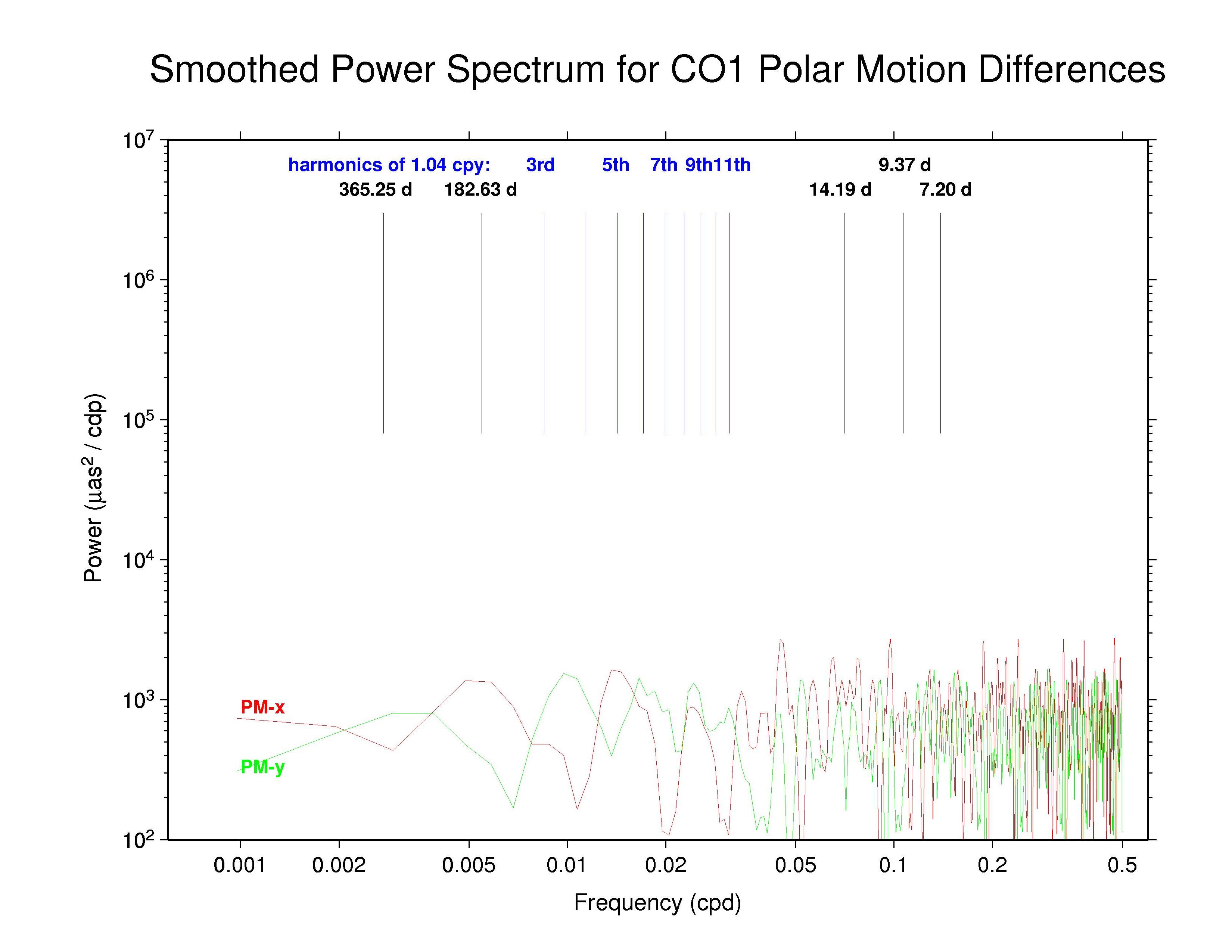
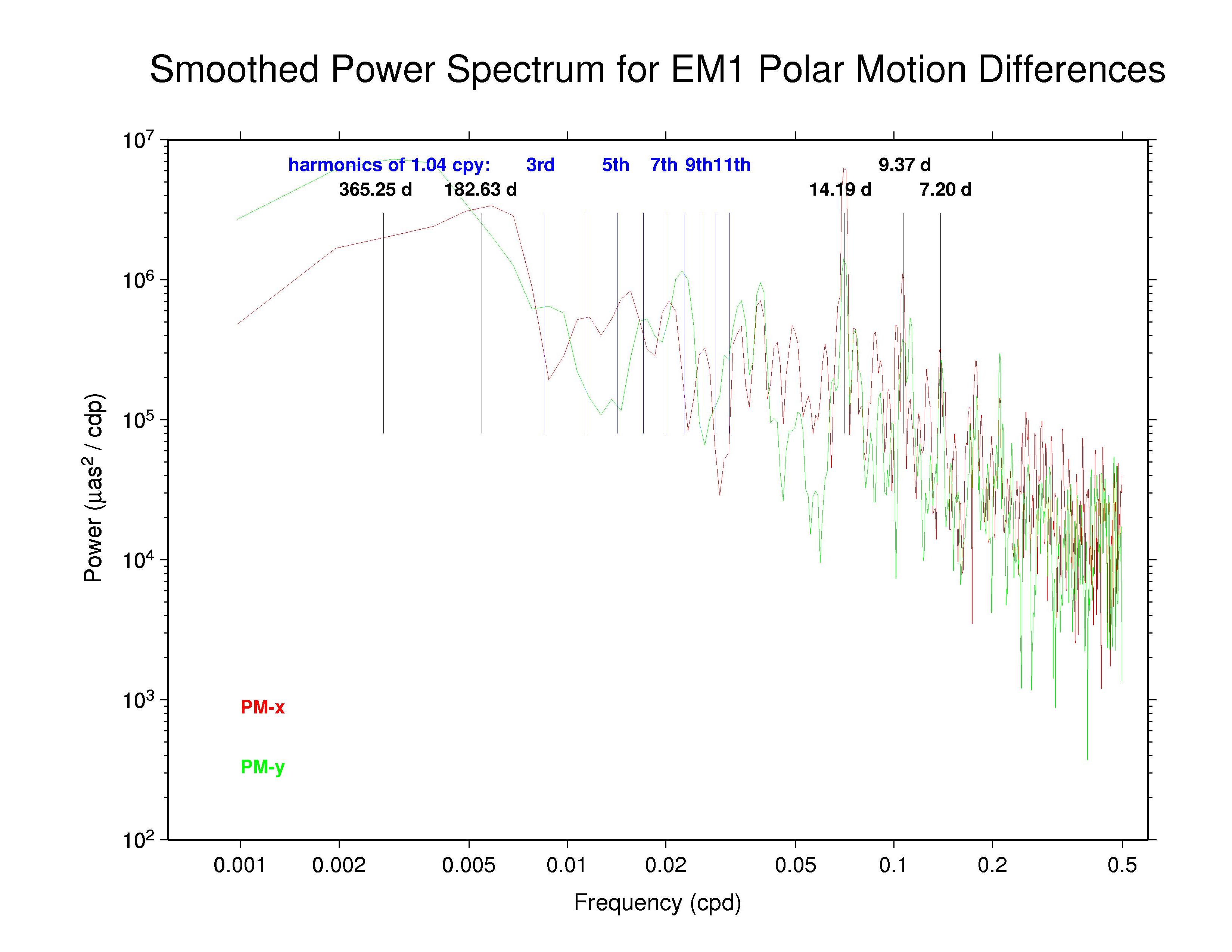
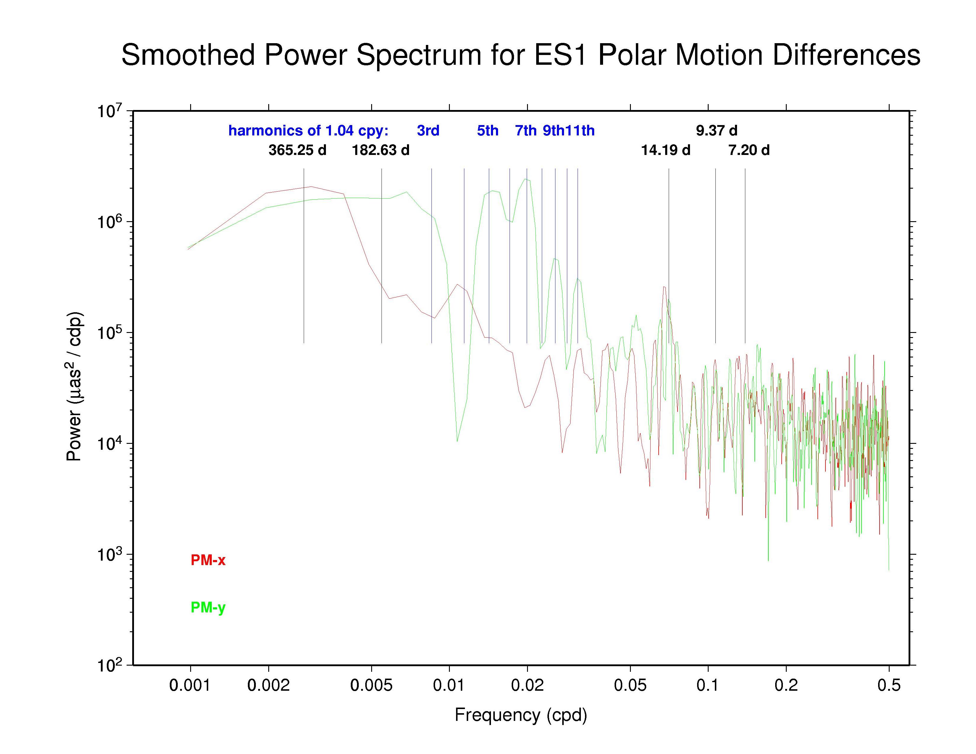
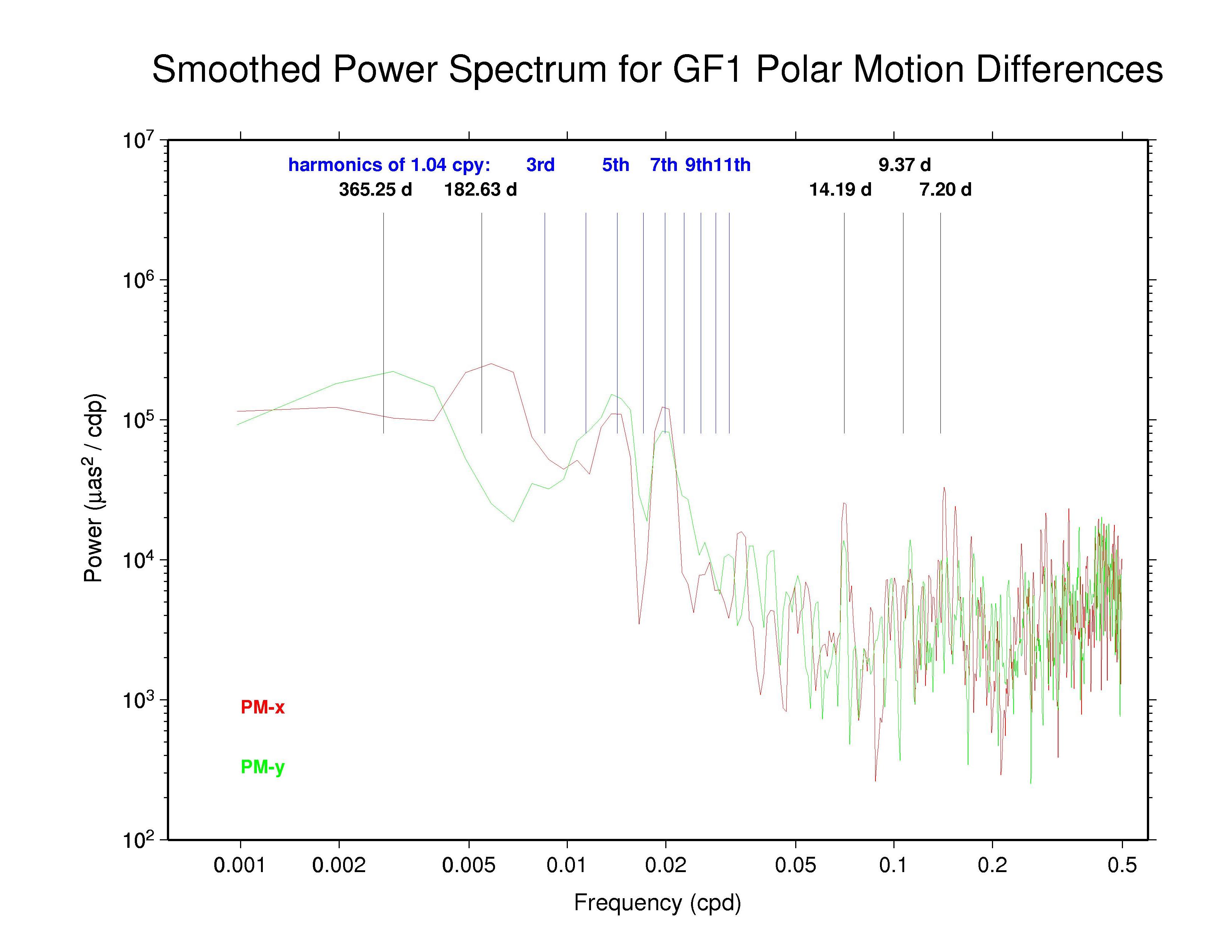
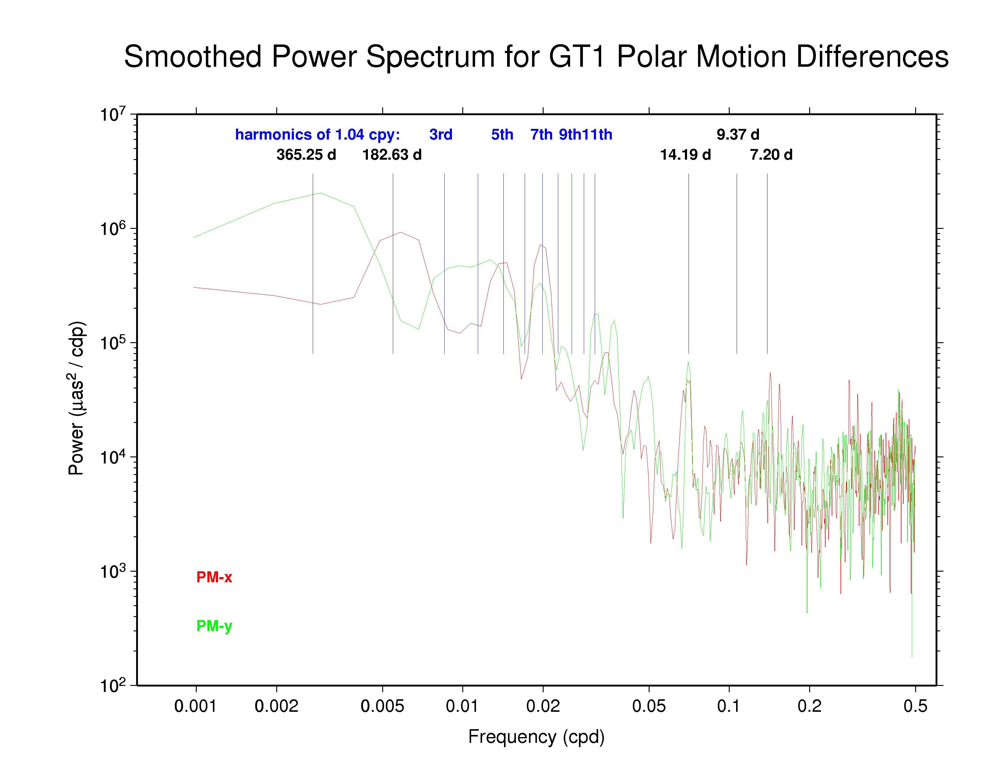
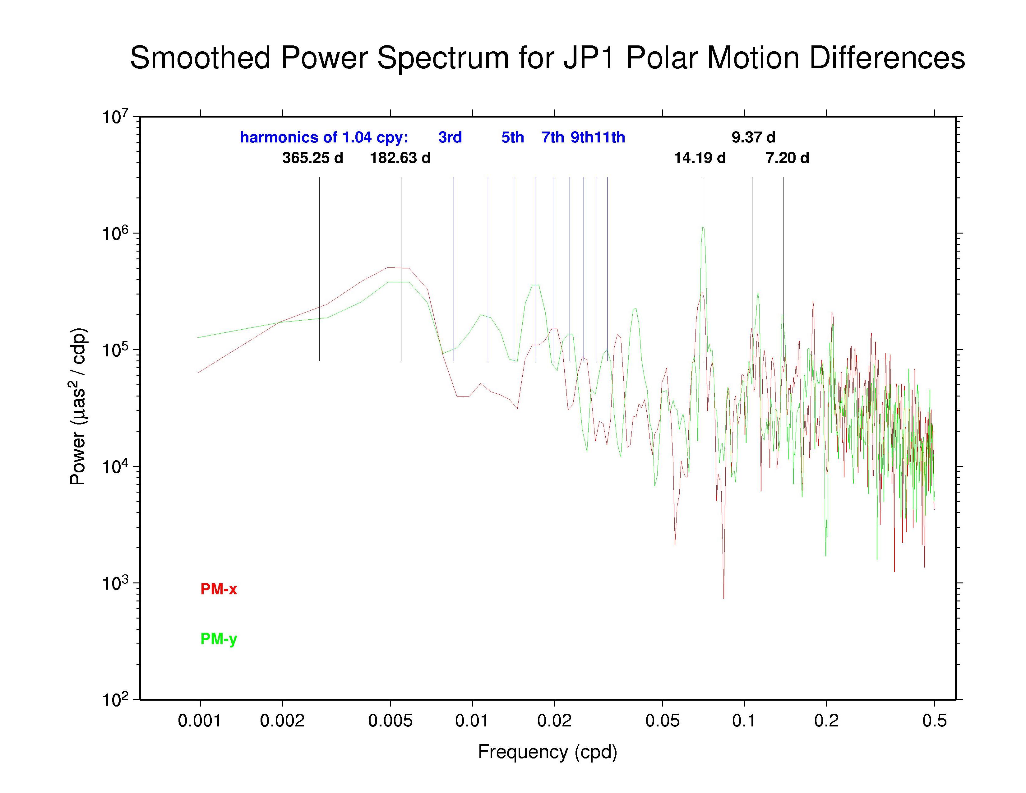
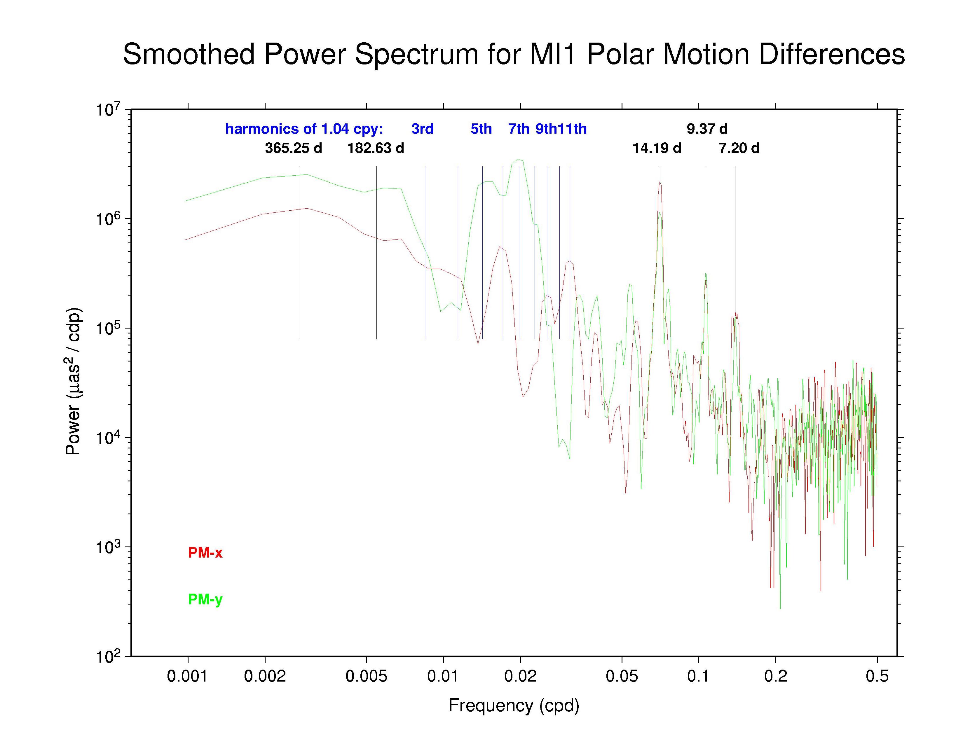
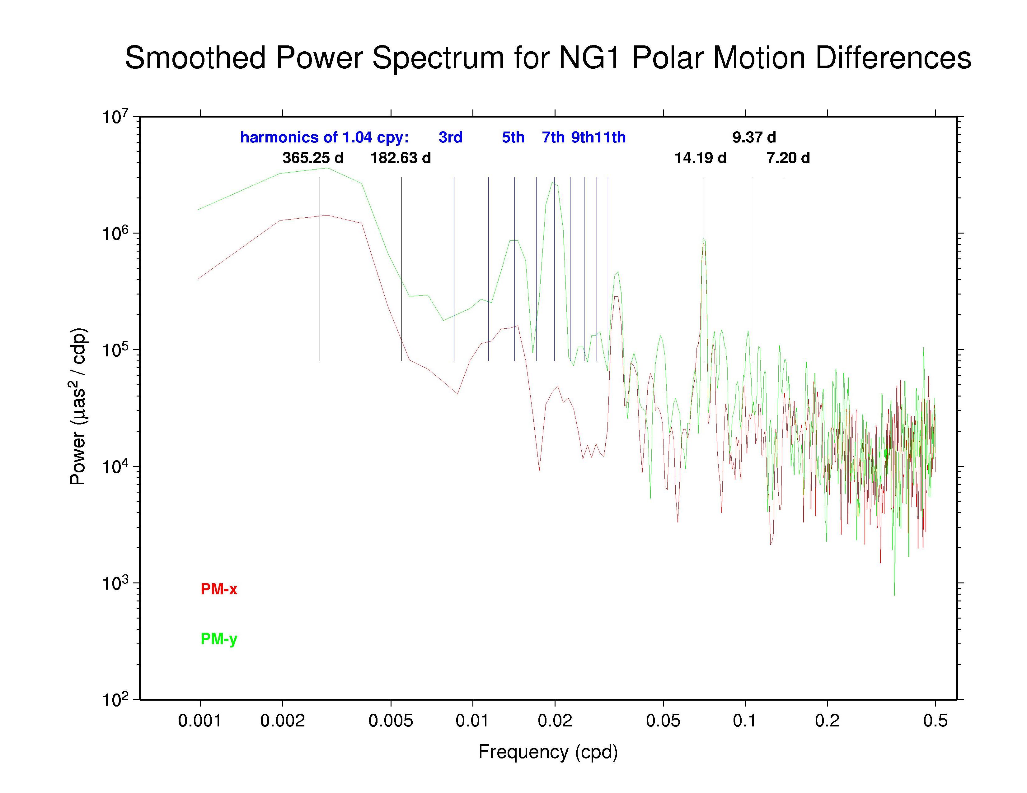
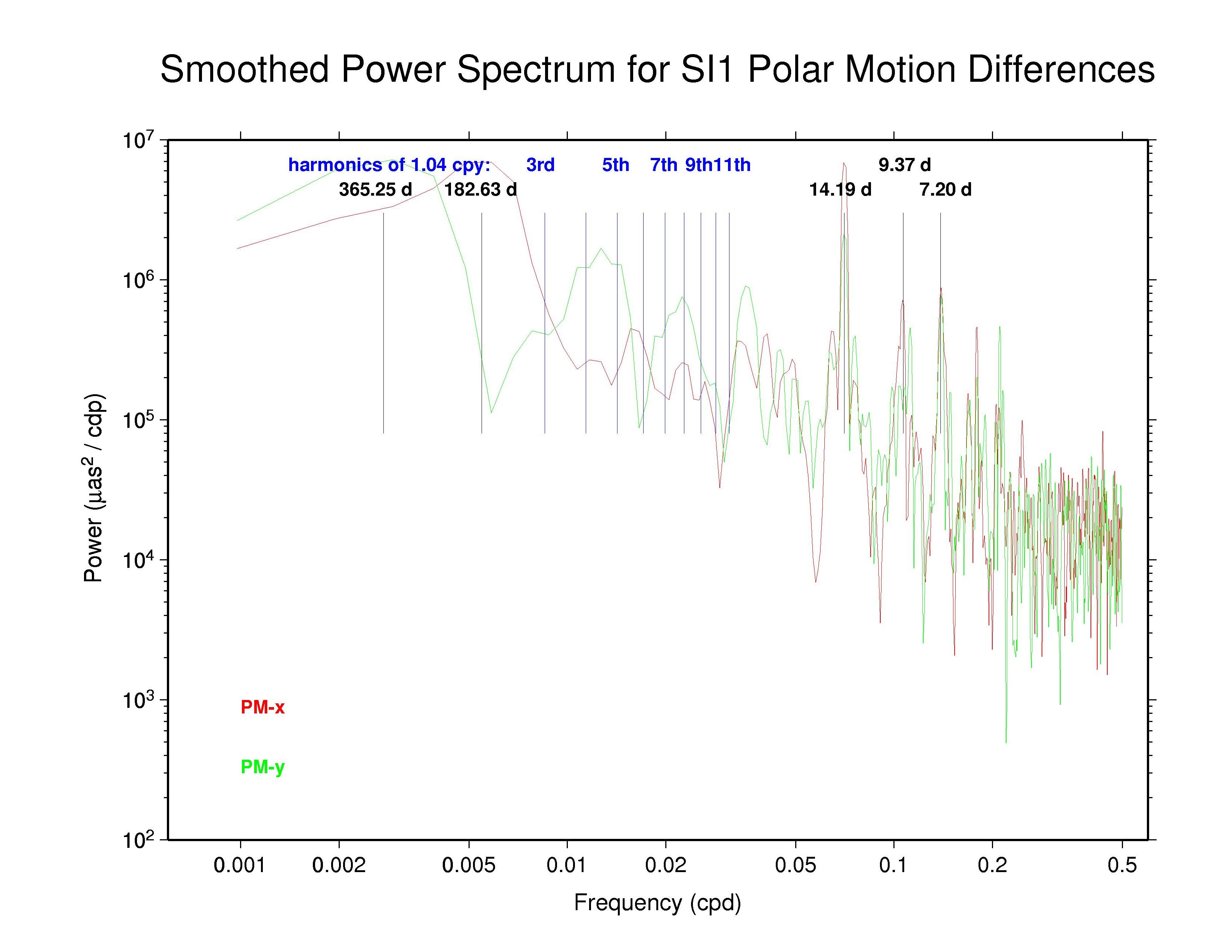
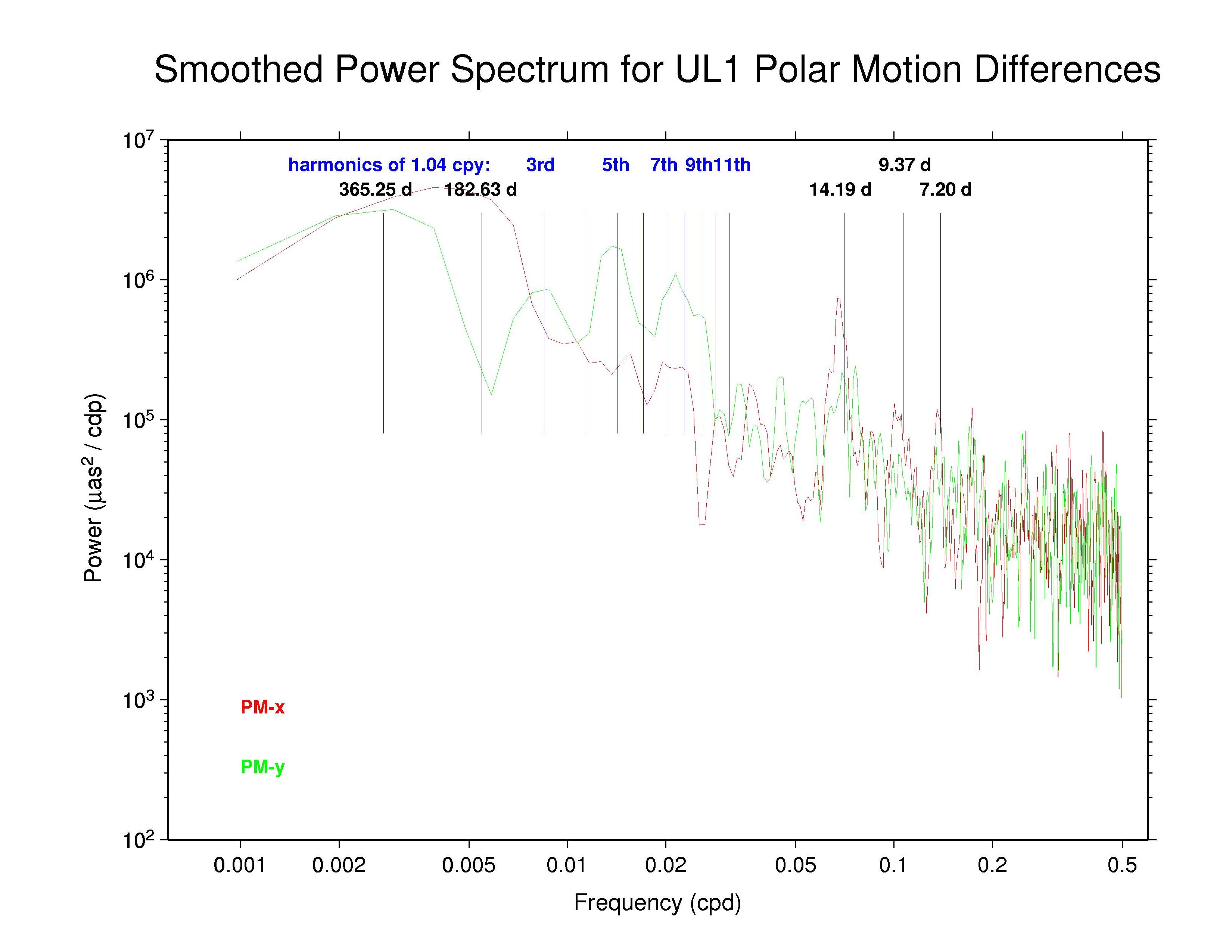
Spectra of the day-boundary differences in polar motion are plotted below, using red for the x component and green for the y component. In each case a boxcar filter has been used to smooth across each three adjacent frequencies. Some interesting spectral lines are also marked in each plot.
 IGS —
ps file IGS —
ps file
|
 CODE —
ps file CODE —
ps file
|
 EMR —
ps file EMR —
ps file
|
 ESA —
ps file ESA —
ps file
|
 GFZ —
ps file GFZ —
ps file
|
 GTZ —
ps file GTZ —
ps file
|
 JPL —
ps file JPL —
ps file
|
 MIT —
ps file MIT —
ps file
|
 NGS —
ps file NGS —
ps file
|
 PDR —
ps file PDR —
ps file
|
 SIO —
ps file SIO —
ps file
|
 ULR —
ps file ULR —
ps file
|
The table below summarizes the main features that can be observed in the spectra of the AC polar motion discontinuity plots above. The ubiquity of the 14.2 d line reminds us that Kouba (2003) showed that this can be an alias of any error in the adopted subdaily O1 tidal EOP model beating against the IGS 24-hr processing interval. Aliased subdaily tidal lines are considered in more detail below. Kouba (unpublished) previously showed also that errors in the prograde fortnightly nutation model, at 13.66 d, which is among the largest modified terms in the IAU 2000 nutation model compared to the IAU 1980 model, will alias into a retrograde 13.66 polar motion rate error. The latter error is not readily apparent. (Note that the spectral resolution of the plots above is about 0.2 d in the fortnightly band.)
Also seen in the plots above and the table below are broad peaks near the harmonics of the 1.040 cpy draconitic year of the GPS constellation. Ray et al. (2008) found a comb of harmonics of the 1.040 cpy GPS year fundamental tone in time series of ITRF2005 position residuals, extending up to at least the 6th multiple; the exact mechanism linking possible orbital errors with the station position residuals was not identified. It is therefore not surprising to see similar GPS year harmonics in the IGS polar motion difference spectra. What is distinctive in this case, though, is that the most prominent harmonics are usually the odd multiples and the strongest ones mostly seem to be the 5th and 7th tones. This behavior constrasts with the day-boundary discontinuity spectra of the repro1 orbits where the even draconitic harmonics, especially the 2nd (presumbly mixed with semi-annual errors related to eclipse seasons), 4th, and 6th, are most commonly seen. The JPL PM-y component differs from the usual pattern in having stronger even harmonics. The COD and PDR spectra are featureless because the strict day-boundary continuity conditions that were applied (and have not been removed here for PDR).
| Features in Spectra of AC Day-boundary Polar Motion Discontinuities | ||||||
| AC | component | annual | semi-annual | tidal alias lines | 1.040 cpy harmonics | |
| IGS | PM-x | Y | - | 14.2, 9.4? | 5th, 7th?, 9th?, 12th? | |
| PM-y | Y | - | 7.2? | 5th, 7th | ||
| COD | PM-x | - | - | - | - | |
| PM-y | - | - | - | - | ||
| EMR | PM-x | ? | Y | 14.2, 9.4, 7.2? | ? (noisy) | |
| PM-y | Y | - | 14.2, 9.4?, 7.2? | ? (noisy) | ||
| ESA | PM-x | Y | - | 14.2? | - | |
| PM-y | ? | ? | 14.2? | 3rd?, 5th, 7th, 9th, 11th | ||
| GFZ | PM-x | - | Y | 14.2, 7.2? | 5th, 7th | |
| PM-y | Y? | - | 14.2 | 5th, 7th | ||
| GTZ | PM-x | - | Y | 14.2, 7.2? | 5th, 7th | |
| PM-y | Y | - | 14.2 | 3rd?, 5th?, 7th, 11th | ||
| JPL | PM-x | - | Y | 14.2, 9.4? | 7th?, 9th? | |
| PM-y | - | Y | 14.2, 9.4?, 7.2? | 4th, 6th 8th 11th? | ||
| MIT | PM-x | ? | ? | 14.2, 9.4, 7.2 | 6th, 9th?, 11th | |
| PM-y | ? | ? | 14.2, 9.4, 7.2 | 5th, 7th | ||
| NGS | PM-x | Y | - | 14.2 | 5th?, 7th?, 12th? | |
| PM-y | Y | - | 14.2 | 5th, 7th 12th? | ||
| PDR | PM-x | - | - | - | - | |
| PM-y | - | - | - | - | ||
| SIO | PM-x | - | Y? | 13.9, 7.0, 4.7, 2.8, 2.0 | - | |
| PM-y | - | - | 2.8?, 2.0 | - | ||
| ULR | PM-x | ? | Y | 14.2?, 9.4?, 7.2? | - | |
| PM-y | Y | - | - | 5th, 7th? | ||
The previous table of aliased subdaily tidal lines by Kouba (2003) has been expanded below to include many more waves, based on values provided Richard Ray (private communication March 2009).
Kouba's analysis previously identified the important O1 aliased feature at 14.19 d, as well as possible lines due to the Q1 wave at 9.37 d, the N2 wave at 9.62 d, and the M2 wave at 14.75 d. He also noted that K1 and P1 errors are expressed at an annual period. Of these, the annual, 14.2 d, and 9.4 d peaks are all seen in at least some of the day-boundary discontinuity spectra, though the 9.4 d peak is not as prominent as the other two. The occasional peaks near 7.2 d were not noted by Kouba as an alias of any subdaily tidal errors. However, in Richard Ray's expanded alias table (below) this can be interpreted as an error in the σ1 subdaily tide. In the IGS combined PM-y spectrum and the spectra of some ACs there are even possible indications of a distinct feature near 29.8 d (0.0336 cpd), which might be attributable to errors in the modeled M1 tide.
Since all ACs claim to apply the IERS 2003 subdaily EOP tide model except for EMR, which continues to use the older 1996 model, we conclude that the 14.2 d, probably the 9.4 and 7.2 d, and possibly the 29.8 d spectral peaks reflect residual errors in that model. This corresponds to significant errors in the subdaily tidal model values for, respectively: O1; Q1 and/or N2; and σ1, 2Q1, 2N2, and/or μ2. While one could readily expect various different types of non-tidal errors near the annual period, contributions also from K1 (especially), P1, and T2 errors cannot be excluded. (Discussions are underway with Richard Ray about generating an updated subdaily EOP tide model, which could be tested using the IGS polar motion rate discontinuity results.)
| Expected Alias Peaks due to
Errors in Subdaily EOP Model (from Richard Ray) | ||
| Tide wave | Period (hr) | Alias period (d) |
| 2Q1 | 28.01 | 7.0 |
| σ1 | 27.85 | 7.2 |
| Q1 | 26.87 | 9.37 |
| ρ1 | 26.72 | 9.8 |
| O1 | 25.82 | 14.19 |
| M1 | 24.83 | 29.8 |
| P1 | 24.07 | 365.2 |
| S1 | 24.00 | infinity |
| K1 | 23.93 | 365.2 |
| ψ1 | 23.87 | 182.6 |
| φ1 | 23.80 | 121.7 |
| J1 | 23.10 | 25.6 |
| OO1 | 22.31 | 13.2 |
| MNS2 | 13.13 | 5.8 |
| 2N2 | 12.91 | 7.1 |
| μ2 | 12.87 | 7.4 |
| N2 | 12.66 | 9.62 |
| ν2 | 12.63 | 10.1 |
| M2 | 12.42 | 14.75 |
| λ2 | 12.22 | 27.6 |
| L2 | 12.19 | 31.8 |
| T2 | 12.02 | 365.3 |
| S2 | 12.00 | infinity |
| K2 | 11.97 | 182.6 |
| Send comments to Jim Ray | (updated 12 May 2009) |