FEATURES
OF DATA
ANALYSES
(new
models
highlighted
in red)
|
 IERS Conventions
(2010) — generally should be implemented
IERS Conventions
(2010) — generally should be implemented
use IGb08 reference frame (aligned to ITRF2008)
- background information in
IGS Mail #6354
- implemented in IGS operational
solutions starting
GPS week 1632
- reference frame file is
IGb08.snx
in SINEX format
- with associated discontinuities file
soln_IGb08.snx
tabulated in SINEX format
- ACs are recommended to use the
IGb08 "core"
subnetwork to realize their frame orientation via a no-net-rotation
(NNR) condition
- updates to IGb08 (i.e., IGb08) and igs08.atx
(i.e., igb08.atx) are pending and will likely form the basis of repro2
use updated igs08.atx "absolute" antenna calibrations
- includes phase center offsets (PCOs) &
direction-dependent phase center variations (PCVs) for both satellite
transmit & ground receive antennas
-
background information in IGS Mails
#5189,
#6355,
& #6374
- implemented in IGS operational
solutions starting
GPS week 1632
- current antenna calibration file is
igs08.atx in
ANTEX format
time argument
- as usual, GPS time (a realization of
terrestrial time, TT) is used for all output analysis products
clock center-of-network (CLK:CoN) convention
- AC clocks must be delivered with apparent
geocenter motion removed by, for example, using your AC adjusted orbits and
fixed IGb08 station coordinates at epoch of observations--this is the
so-called clock center-of-network (CLK:CoN) convention in the SP3 files
introduced by G. Gendt; more details at:
—
position paper from 2004 IGS Workshop, esp. Recommendations 10 & 11
ftp://igs.org/pub/resource/pubs/04_rtberne/Session1_1.pdf
—
and resulting action for SP3 file comment lines
http://acc.igs.org/sp3-comments.html
P1-C1 satellite code biases
phase wind-up correction
- RHC phase rotations due to geometric
changes should follow the model of J.T. Wu, S.C. Wu, G.A. Hajj, W.I.
Bertiger, and S.M Lichten ("Effects of antenna orientation on GPS
carrier phase", Manuscripta Geodaetica, 18, 91-98,
1993)
- the Wu et al. model was
conveniently restated by J. Kouba (2009) in his
"A Guide to Using
IGS Products"; see section 5.1.2
yaw attitude variations
- changes in GPS satellite orientation
during eclipse periods will follow the model of
J. Kouba (2009) or equivalent
- this is especially important for
consistent satellite clock estimates
- new yaw-attitude model under
development for GPS Block II-F satellites by
F. Dilssner (2010)
- new yaw-attitude model for GLONASS-M
satellites published by
F. Dilssner (2010)
- to implement these models, J. Kouba
(2011, private communication) has provided the Fortran routine
eclips.f (version updated January
2014) together with a
EclipseReadMe.pdf file containing
usage information
— note that the August 2011 version has been updated to use
yaw rates for the Block II/IIA satellites during the period
1996-2008 that are based on weighted averages of the JPL repro1
yaw-rate solutions; see
yrates.pdf for details
— the September 2011 version has been updated to fix a bug
related to night maneuvers for IIF satellites at high beta angles
— note also that Block II/IIA shadow eclipsing model is
valid only after 5 November 1995 when the orientation control of
the satellites was updated to be biased by +0.5 degrees in order
to produce shadow behavior that is predictable; prior to that
date, shadow-crossing data should not be used
— the December 2013 version has been updated to correct the
Block IIF shadow crossing according to the U.S. AF documentation, which
states that the shadow crossing yaw rate is computed from the shadow
start and end nominal yaw angles and the shadow crossing time interval.
Also included in the December update are models for recently noticed
anomolous IIF and IIA noon turns for small negative (>-0.9 deg)
and positive (< 0.9 deg) sun (beta) angles, respectively. So the now
current version should correctly model eclipsing of IIA/IIF/IIR and
GLONASS satellites. More info is provided in
EclipseDec2013Update.pdf.
— the December 2013 version has been updated to fix a bug
related to noon turn end for a small positive sun beta angle (<0.9 deg)
- utilization of the yaw attitude model
should consider changes in the phase wind-up correction (see section
above) as well as changes in the location of the antenna phase center
relative to the satellite center-of-mass due to non-zero X offsets for
some spacecraft; see "A
Guide to Using IGS Products" by J. Kouba (2009) for details; note
that data from Block IIA GPS satellites should also be deleted for an
interval following shadow exits
modeling of orbit dynamics
- rotational errors are a major limit
to the accuracy of all IGS orbit products; see:
— J. Ray & J. Griffiths,
2010
— J. Ray & J. Griffiths,
2011
- these are probably due mostly to
shortcomings of present once-per-rev empirical parameterizations
commonly used to absorb unmodeled accelerations & lead to the
flicker noise background documented in station coordinate time
series
- errors in the IERS model for subdaily
EOP variations contribute also & both factors lead to aliased orbit
errors at draconitic harmonics that contaminate all IGS products
(see J. Ray & J. Griffiths,
2011)
- other errors, especially in the IERS
model for subdaily EOP variations, also contribute to subdaily orbit
rotation errors that alias to annual, ~29, ~14, ~9, & ~7 days when
sampled daily
- reflected (albedo) & retransmitted
radiation from the Earth may cause scale (1 - 2 cm) &
translational effects at GNSS altitudes; see:
— C.J.
Rodriguez-Solano, 2009
— U. Hugentobler
et al., 2009
— C.
Rodriguez-Solano, 2011et al., 2011
— website at
Technische Universit�t M�nchen (TUM)
- a recommended model for these effects,
in the form of Fortran source code developed within the scope of
the IGS Orbit Modeling Working Group, is available for
download here (30 March 2011)
— an update of the routine
ERPFBOXW.f was posted by C. Rodriguez-Solano (21 September 2011)
to account for Block-dependent transmitter thrust values for the
GPS satellites (updated again 13 June 2012 for bug fixes)
— a compilation of the calculated & estimated GPS transmit
power levels is posted here
- any albedo models might be proposed
or implemented should be carefully evaluated for their impacts on
other parameter estimates (e.g., on the terrestrial reference frame)
EGM2008 geopotential field now recommended
- updated values for time-variations
of low-degree coefficients given in IERS Conventions (2010)
Chapter 6
- new model for the mean pole trajectory
given in IERS Conventions (2010) section 7.1.4 should be used for
both geopotential and station displacement variations; see eqn
(7.25) & Table 7.7
- geopotential ocean tide model updated
for FES2004 model
- new model introduced for ocean pole
tide (also for station displacements)
-
[OPEN TOPIC] impacts on IGS products from seasonal variations in geopotential
tidal displacements of station positions
- current recommendations for solid
Earth & ocean tidal loading should already be implemented
— site-dependent
load coefficients recommended using FES2004 ocean tide
model
— corrections for counter-balancing center-of-mass motion of
the solid Earth should be included in site coefficients
("Do you want to correct your loading values for [geocenter]
motion?" YES)
—
whole-Earth center-of-mass corrections should also be
applied in generating SP3 orbits as described in
IERS Conventions (2010) section 7.1.2
- new model for the mean pole trajectory
should be used for pole tide correction; see IERS Conventions (2010)
eqn (7.25) & Table 7.7
- ocean pole tide loading model given
in IERS Conventions (2010) section 7.1.5
- [NO LONGER RECOMMENDED] new model for S1 & S2 atmosphere
pressure loading given in IERS Conventions (2010) section 7.1.3
— effect is small but aliases into GPS orbit parameters
otherwise
— note center-of-mass frame corrections for SP3 orbits
(similar to ocean tidal loading); see Table 7.6
no non-tidal loading displacements should be applied to station
positions
- since a key geoscience application of
IGS station time series is to monitor non-tidal loading effects,
these should be fully retained in products unless 1) it can
be shown that there are strong reasons not to do this and 2) any
corrections removed a priori are accurately known and can
also be restored a posteriori
- other reasons not to apply
a priori modeled loading estimates to raw GNSS data are
(see also Ray et al. 2007):
— global circulation models do not reliably account
for dynamic oceanic response for periods < ~10 days
— discrepancies among global circulation models & among load
computations are significant compared to geodetic
accuracies (see e.g.,
T. van Dam,
2005 &
L. Koot et al., 2006)
— topographic corrections, which can exceed 100% of the total
effect in mountainous areas, are not properly modeled by
operational services
(T. van Dam
et al., 2010)
— models must be free of tidal effects (since these are
handled separately), which is usually not the case
— long-term model biases, such as lack of overall mass
conservation, will corrupt reference frame
— inability to remove or modify models applied by ACs at the
observation level
— significant discrepancies remain between non-linear GNSS
observations & models, even at annual periods, implying
important systematic errors yet to be understood (see, e.g.,
X. Collilieux
et al., submitted 2011)
- if useful, non-tidal loading corrections
can be applied in long-term stacking of GNSS weekly frames to minimize
possible aliasing of Helmert parameters
— see, e.g.,
X. Collilieux
et al., submitted 2011
— this use is efficient & fully reversible, unlike
corrections at the observation level
- due to the level of high-frequency
non-tidal atmosphere loading variance, it is necessary to move from
weekly to daily frame integrations in order to fully preserve loading
signals in IGS position time series without significant attenuation
— this change was made operationally starting with Wk 1702 products
— this can be seen in the plot below, which shows dUp power
spectra for atmospheric pressure loading at 415 globally
distributed IGS stations computed from the NCEP reanalysis
pressure fields (courtesy of T. van Dam, 2011)
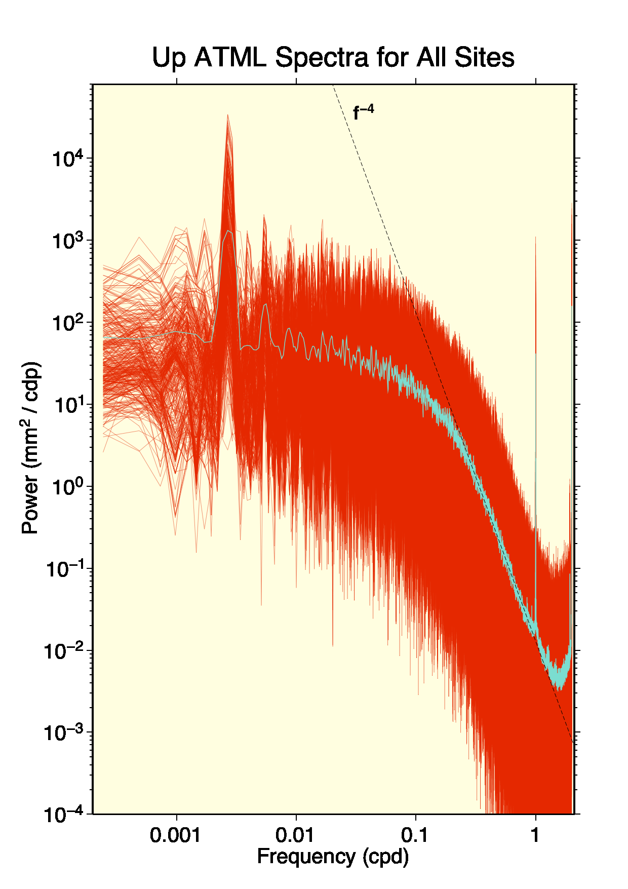
— the stacked mean PSD for this ensemble of stations is shown
by the turquoise line, which follows a power-law with spectral
index of -4 for frequencies >0.4 cpd (ignoring the strong
S1 & S2 tidal lines; the S2 line is broadened by being at
the Nyquist sampling limit)
— the fit for the mean atmosphere pressure loading trend from
0.4 cpd upward (but omitting the tidal bands around 1.0 &
from 1.13 cpd onward) is approximately:
PSDUp = 0.013 mm2/cpd * f -4
indicated by the dotted line in the plot above
— integrating this power law from 1/1 cpd to infinity & from
1/7 cpd to infinity, assuming the same -4 power law extends
to the highest possible frequencies, gives these variances,
respectively:
Var (1/1 -> inf)Up = 0.00433 mm2
Var (1/7 -> inf)Up = 1.486 mm2
or equivalently these scatters, respectively:
RMS (1/1 -> inf)Up = 0.066 mm
RMS (1/7 -> inf)Up = 1.219 mm
— for a GPS dUp measurement with a basement error of about
2.2 mm for weekly observations (as found from the IGS repro1
results), one must expect daily measurements to have errors
no smaller than sqrt(7) times larger if there are no
temporal error correlations (higher otherwise) or about
5.8 mm; so the actual atmospheric pressure dUp loading
variations are much smaller than the GPS detection limit
for 1 d intervals (by about two orders of magnitude on
average) but the average load variations are within a factor
of ~2 of the GPS WRMS noise floor for weekly dUp integrations
& can even exceed the GPS noise floor at some extreme
stations (considering the spatial variation in PSD spans
about a factor of 10 upward and downward, or equivalently a
factor of 3 to 4 in RMS)
— consequently, this suggests that there is some loss, on
average, in GPS sensitivity to atmosphere loading with the
present IGS weekly integrations when load corrections are
not applied, but this would not be the case with daily
frame integrations
tidal EOP variations
- most current models & recommendations
should already be implemented
- this includes the subdaily polar motion
libration terms introduced in 2005 & previously called "high-frequency
nutation", which can be computed using fortran routines PMsdnut.f or
PMSDNUT2.f
- key exception is the addition of UT1
libration effects, introduced in late 2009
- see IERS Conventions (2010) Table 5.1b
for coefficients of 11 largest semidiurnal UT1 libration terms or
use the new fortran routine
UTLIBR.F
from A. Brzezinski
- note that the maximum UT1 libration
effect is 105 µas (peak-to-peak) or 13 mm at GPS altitude,
which probably aliases strongly into the orbit parameters
- standard IGS Earth rotation
parameterization should be used, with daily (noon) estimates for
the x,y coordinates of polar motion, their time derivatives over
the 24 hr surrounding each noon, & (nominal) length-of-day (LOD)
variations over the 24 hr surrounding each noon
- each set of daily ERPs should be
determined freely, without any a priori or continuity
constraints
tropospheric propagation delays
- for details, refer to
IERS
Conventions (2010) section 9.2
- a priori meteorological data
sources:
[1] local sensor met files (which however are only available for a
few sites), or
[2] the fortran routine GPT2.f returns
location- & season-dependent values for local pressure,
temperature, temperature lapse rate, water vapor pressure,
hydrostatic and wet mapping function coefficients ah & aw, and
geoid undulation based on a 5 x 5 degree gridded fit to a long
history of ECMWF fields; this updated version gives much better
spatial and temporal resolution than the prior GPT.f model
available at the IERS Conventions website; please refer to
the
README comments for further
information; the associated external grid file is available
here & should be placed in the
directory where the routine is run or else the subroutine open
call modified
[3] retrieved from a numerical weather model, as for the ECMWF global
values provided by the
service at the
Technical University of Vienna in the form of gridded
hydrostatic zenith delays; for details, see the
README
file
- a priori hydrostatic delays
in the zenith direction should be computed from the surface pressure
from any of the sources above according to the formula of Saastamoinen
(1972) as given by Davis et al. (1985) & shown as
eqn
(9.11) in IERS Conventions (2010) Chapter 9
- a priori wet delays in the
zenith direction can also be computed provided that the local
temperature and water vapor pressure are known (see above):
— a fortran routine for this computation is available at
WETSAAS.f
— the fortran routine WETPP.f
might be helpful to convert between relative humidity and
water vapor partial pressure
- using the sum of the a priori
hydrostatic and wet zenith delays will ensure that the
tropospheric parameter adjustments that are more nearly
zero-mean
— a test at NGS using a week of data from about 235 globally
distributed stations found that using GPT2 for
a priori meteo values improved the residual zenith
tropo delay adjustments from 42 +/- 64 mm (assuming a
relative humidity of 0.50 everywhere) to 3 +/- 54 mm
- a priori azimuthally symmetric
line-of-sight delays should be computed using either:
- a priori asymmetric
line-of-sight delays caused by the mean troposphere distribution
(represented by a spherical harmonic expansion to degree and order 9)
can be evaluated using the fortran routine
APG
— note that the north & east gradients from this routine
should be used with the gradient model by G. Chen &
T.A. Herring ("Effects of atmospheric azimuthal asymmetry
on the analysis of space geodetic data", J. Geophys.
Res., 102(B9), 20,489-20,502, doi:
10.1029/97JB01739, 1997), also described in
APG
— note also that test results using the APG model have not
verified its usefulness, so it is not recommended for
general adoption at this time
- note that using the simpler GPT2
routine (with VMF1_HT) rather than more realistic a prioris
derived from in situ data or numerical weather models can
partially compensate for sub-seasonal atmospheric pressure loading
effects at a level probably smaller than ~1 mm in annual height
variation (see
J. Kouba, 2009 &
P. Steigenberger
et al., 2009); this effect arises due to systematic
limitations of the GPT2 model that fail to capture the full measure
of spatial and temporal variations of the troposphere (together with
small differences in the dry & wet mapping functions, which are very
sharp functions of elevation cutoff angle); consequently, the
magnitude of this compensation effect is a strong function of the AC
elevation cutoff angle; in this respect note also that the
Steigenberger et al. analysis included GPS data with
elevation angles down to 3 degree (with elevation-dependent
weighting); ACs with higher elevation cutoff angles will experience
smaller loading compensation
- but note further that ray-tracing of
direct a priori slant delays using spatially & temporally
high-resolution troposphere models should be superior, in principle,
but sufficient global models are not yet available; however, it has
not been found so far that residual troposphere parameters can
be eliminated from space geodetic solutions, a step that would bring
significant precision improvements if the slant delays can be
determined accurately enough
- residual tropospheric delays should be
parameterized in the GNSS data analysis on the assumption that they
are predominantly due to unmodeled variations in the wet component
of the troposphere zenith delay (that is, using wet mapping function
partials) as well as unmodeled azimuthal gradients
— GNSS data are sensitive to zenith delay changes over
intervals as short as the observation sampling, but
parameterization at hourly intervals is much more
efficient & usually satisfactory
— a minimal gradient parameterization involves one N-S & one
E-W parameter at the beginning & end of each day of data
for each station, with continuous linear variation during
the day
— the Chen-Herring (1997) gradient mapping function is
recommended; see updated
IERS
Conventions (2010) section 9.2:
mg(e) = 1 / [sin(e)tan(e) + 0.0031]
where "e" is the observation elevation angle. Unlike other
gradient mapping functions, this one is not affected by a
singularity at very low elevations & should also be used
with the APG a priori gradient model.
— for gradient estimation, an elevation cutoff angle no higher
than 10 degrees is recommended; otherwise station height
accuracies will suffer
— a priori parameter constraints are not needed & are
strongly discouraged
higher-order ionospheric corrections
- for details, refer to
IERS
Conventions (2010) section 9.4
- a software package has been developed
by M. Hernandez Pajares & colleagues to compute the 2nd order
ionosphere correction; it is available at
this site
- the software is entirely new, with
contributions & debugging from an informal working group of volunteers
- only the 2nd order correction, which
is larger & for which there is a clear consensus on how it should be
applied, is included currently; additional higher-order terms can be
incorporated in the future
analysis constraints
- a limitation in IGS operational &
repro1 products is the application of unremovable constraints by
some ACs (see
R. Ferland, 2010)
- unremovable continuity constraints,
for example, can act as biased filters & cause significant signal
distortions (see
J. Ray, 2008)
- these can be particulary insidious
when applied to pre-reduced parameters, such as orbit estimates,
& are especially difficult to justify for GNSS processing where
almost every parameter is highly observable
- consequently, some AC contributions
are routinely excluded from IGS product combinations
- for repro2, ACs are asked to avoid any
solution over-constraints, applying pre-removed or unremovable
constraints no tighter than noise levels & ensuring that any other
constraints are strictly removable -- see reprocessing recommendations
on p. 10 of the
IGS 2010 Workshop in Newcastle
- failure to meet this condition may
force full AC exclusion from the product combinations
self-certification
- each AC will be asked to certify its
compliance with these standards, noting specific areas of
deviation
- all AC metadata errors reported in the
weekly SINEX combination reports should be corrected
- all ACs should also ensure that their
analysis processing summary files at the IGS Central Bureau are
up to date
|